Introduction.

Welcome to a new post about AI in R. In this post, we are going to explore different ways to solve another simple AI scenario included in the OpenAI Gym, the FrozenLake. FrozenLake in a maze-like environment and the final goal of the agent is to escape from it. The environment is a representation of a frozen lake full of holes, the agent has to go from the starting point (S) to the ending point (G) avoiding the holes (H). The trick is that the agent must walk over frozen tiles (F) to reach the ending point. Unfortunately, the agent can’t perform the desired actions accurately when it is walking over a frozen tile, so each time an agent performs one action there is a chance that it ends up moving into an unwanted direction.

The environment is finished when the agent reaches the (G) tile (Reward=1) or when it falls into a hole (Reward=0).

The FrozenLake is represented as a 4x4 grid with the positions numbered from 0 to 15. The (S) is located at the position number 0, the (G) at the position number 15 and the holes are located at positions 5, 7, 11 and 12:

SFFF
FHFH
FFFH
HFFG

Results.

As I did with the CartPole environment I first tested the performance of a random agent because it provides a first impression of the difficulty of the environment and the presence of possible challenges. The performance of an agent executing a random policy looks like this:

The overall efficiency of the random agent is around 0.5%. At a first glance, it might look too low but indeed it’s much higher than the efficacy of the random policy in the CartPole environment. The second good reason why I always try to run a random agent is because it is possible to extract detailed information about actions and how they drive to positive rewards, so it is possible to extract this information to train subsequent agents that can use those experiences to learn from them.

The FrozenLake is a simple environment in which the combination of positions/actions is quite manageable (64 possible combinations of actions/positions, counting holes and goal tiles) so it is possible to implement a kind of decision tree in which we define the falling probabilities for all combinations of positions-actions. It looks something like this:

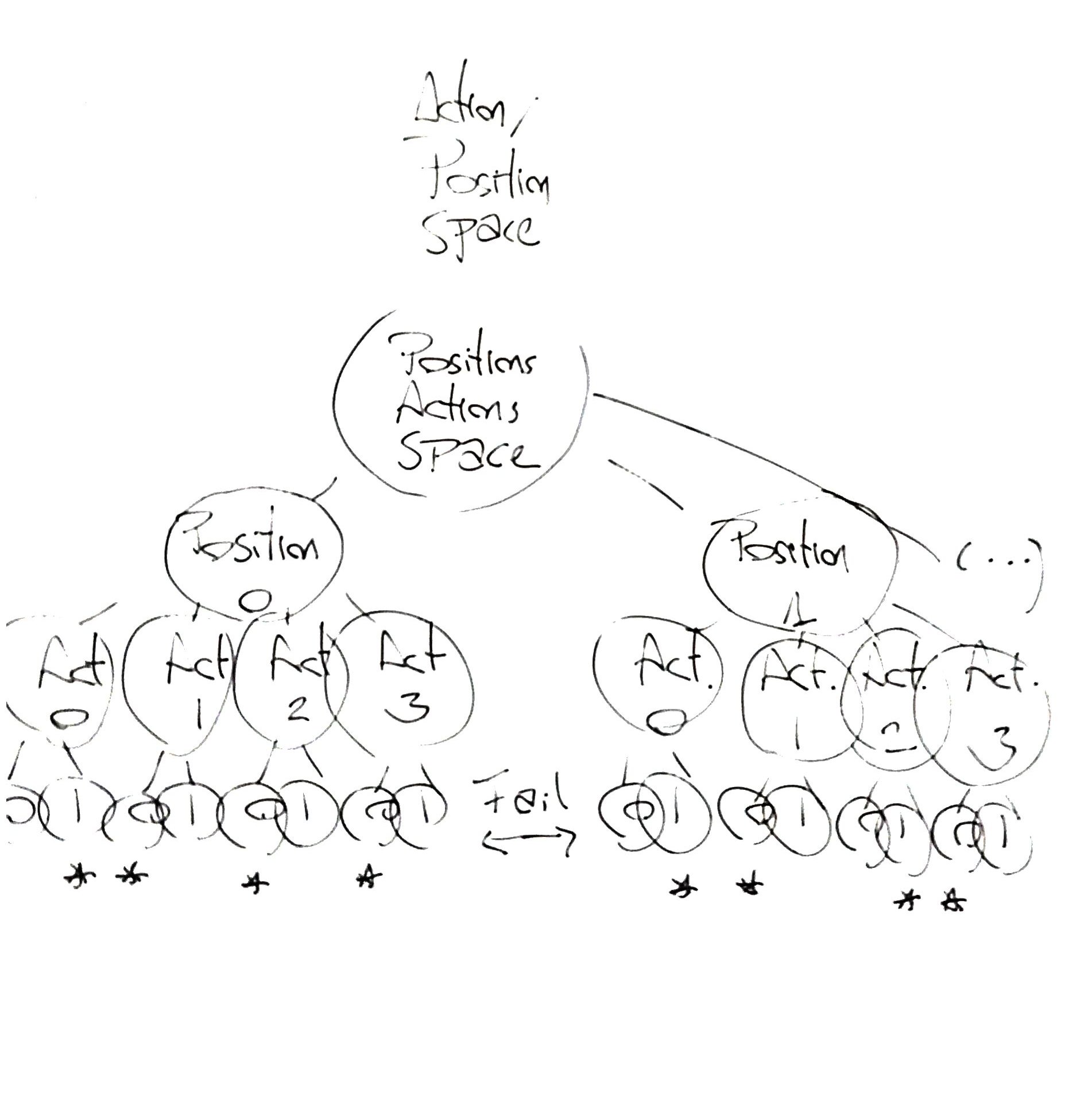
Here is the code to create the tree:

#Growing a tree 
SpaceTree<-expand.grid(c(0:15),c(0:3),c(0,1))
colnames(SpaceTree)<-c("Position","Action","Fail")
SpaceTree$N<-0
SpaceTree$Prob<-0
SpaceTree$Reward<-0
SpaceTree$Length<-0

I have included four additional parameters for each action/position combination to have a more complete view of what is going on.

The tree is going to account for the falling probability (SpaceTree$Prob), the probability of getting a reward when performing that action (SpaceTree$Reward), the number of times the agent has visited the tile (SpaceTree$N) and how many steps the agent takes until the episode is solved (SpaceTree$Length).

Next we fill in those parameters with the values obtained by the random-agent that, as in the CartPole scripts, are stored into the variable dfGod (you can get an updated form of the script here)

for (i in 1:nrow(SpaceTree)) {
  SpaceTree$Prob[i] <- length(dfGod2$Position[dfGod2$Position==SpaceTree$Position[i] &
                                               dfGod2$Action==SpaceTree$Action[i] & 
                                               dfGod2$Fail==SpaceTree$Fail[i]])/
                       length(dfGod2$Position[dfGod2$Position==SpaceTree$Position[i] &
                                               dfGod2$Action==SpaceTree$Action[i]])
  
  SpaceTree$N[i] <-length(dfGod2$Position[dfGod2$Position==SpaceTree$Position[i] &
                                               dfGod2$Action==SpaceTree$Action[i] & 
                                               dfGod2$Fail==SpaceTree$Fail[i]])

  SpaceTree$Reward[i] <- length(dfGod2$Position[dfGod2$Position==SpaceTree$Position[i] &
                                               dfGod2$Action==SpaceTree$Action[i] & 
                                               dfGod2$RewardEp==1])/
                         length(dfGod2$Position[dfGod2$Position==SpaceTree$Position[i] &
                                               dfGod2$Action==SpaceTree$Action[i]])
  
  SpaceTree$Length[i]<-mean(dfGod2$StepMax[dfGod2$Position==SpaceTree$Position[i] &
                                               dfGod2$Action==SpaceTree$Action[i]&
                                               dfGod2$RewardEp==1])  
}

Now that tree/library of actions-fails-rewards is ready, it is possible to use it as the engine to create different policies:

The Reward based policy:

#Action driven by Reward
      PosAct<-subset(SpaceTree, SpaceTree$Position==dfGodN$Position[j] & SpaceTree$Fail==0)
      action <- subset(PosAct,PosAct$Reward == max(PosAct$Reward))
      action <- action$Action
      if (length(action) > 1) action<- action[round(runif(1,min = 1, max = length(action)))]

An agent following this policy searches for the action with the highest probability of solving the environment for the current position. In the case that two or more actions had the same probability of success, the agent randomly selects one of them.

This agent solves the environment 15.4% of the times, that is 30 times better than the random agent.

The Hole avoidance policy:

      #Action driven by hole avoidance
      PosAct<-subset(SpaceTree, SpaceTree$Position==dfGodN$Position[j] & SpaceTree$Fail==1)
      action <- subset(PosAct,PosAct$Prob == min(PosAct$Prob))
      action <- action$Action
      if (length(action) > 1) action<- action[round(runif(1,min = 1, max = length(action)))]

This agent performs the action asociated with the lowest probability of falling into a hole independetly if the agent solves the enviroment or not. The agent would also execute a random selection of actions if two or more actions had the same probability of falling.

The efficiency of this policy is around 42%. This observed increase in the performance is kind of expected since the random-agent provided much more information about actions that lead to a fall in a hole than information about actions that can solve the environment.

The Reward-Hole policy:

PosAct<-subset(SpaceTree, SpaceTree$Position==dfGodN$Position[j] & SpaceTree$Fail==1)
       action <- subset(PosAct,PosAct$Prob == min(PosAct$Prob))
       action <- action$Action[action$Reward == max(action$Reward)]
       if (length(action) > 1) action<- action[round(runif(1,min = 1, max = length(action)))]

Based on the results obtained by the hole-avoider and the reward-searcher, I decided to combine both policies to see if it would be possible to increase the efficiency further. This hole-avoider-reward-searcher agent avoids the actions that drove the random agent to fall into a hole and in case of several actions having the same probability of falling, the agent selects the one with the highest probability of solving the episode. The agent performs surprinsingly well, it solves the enviroment 73.4% of the times. However, I noticed that the agent took a lot of steps to solve the environment (41 steps on average), by introducing a delay in the execution of the code with Sys.sleep() I could explore the behaviour of the agent:

The agent apparently gets stuck at the beginning of the episode and it seems that it can only continue when it randomly ends in an unwanted tile. One could think of this behavior as if the agent were pushing the borders of the FrozenLake to avoid falling. This behavior reminds me of one described in a post called Faulty Rewards in the Wild in which the guys from OpenAI describe something similar.

Next, I tested an agent in which solving the episode was prioritized over avoiding the holes:

PosAct<-subset(SpaceTree, SpaceTree$Position==dfGodN$Position[j] & SpaceTree$Fail==1)
      action <- subset(PosAct,PosAct$Reward == max(PosAct$Reward))
      action <- PosAct$Action[PosAct$Prob == min(PosAct$Prob)]
      if (length(action) > 1) action<- action[round(runif(1,min = 1, max = length(action)))]

This new agent shows a decent performance although it is not as good its sibling’s, only 41.2% of the times the environment is solved. Unfortunately, the agent partially inherited the erratic behavior observed in its sibling.

Reward-Speed policy

PosAct<-subset(SpaceTree, SpaceTree$Position==dfGodN$Position[j] & SpaceTree$Fail==1)
       action <- subset(PosAct,PosAct$Reward == max(PosAct$Reward))
       action <- action$Action[action$Length == min(action$Length)]
       if (length(action) > 1) action<- action[round(runif(1,min = 1, max = length(action)))]

As a solution to fix the erratic behavior observed in some of the agents I implemented a Reward-Speed policy; the agent first tries to maximize the reward and then tries to minimize the number of steps taken. However, this agent only solves the episode 16.7% of the times. This is probably due to the lack of successful experiences in the library of actions/positions as I mentioned before.

Until this point we have seen how it is possible to optimize the use of a library to compile the experiences of the random agent; nevertheless, none of these agents can really learn anything. They need a library of actions and this library could be inaccurate, outdated or very sparse in rewarded episodes. Additionally, it could also be possible to have a library larger than what is necessary. The only way to solve these issues is by creating an agent that can learn as it experiences the environment.

The Self-Learner agent
A self-learner agent needs to store the information that it gets during the different episodes. To do that I have implemented a tree/library at end of every episode to store all the information acquired. The structure of the tree is basically the same as the one implemented for the other agents.

Additionally, a learning curve to make decisions needs to be implemented in a way that if the agent hasn’t visited enough the current position it executes a random action. The more experiences about a position the agent has, the more it relies on its library of experiences. There are many possibilities to implement this idea, but a sigmoidal learning curve looks quite logical to me:

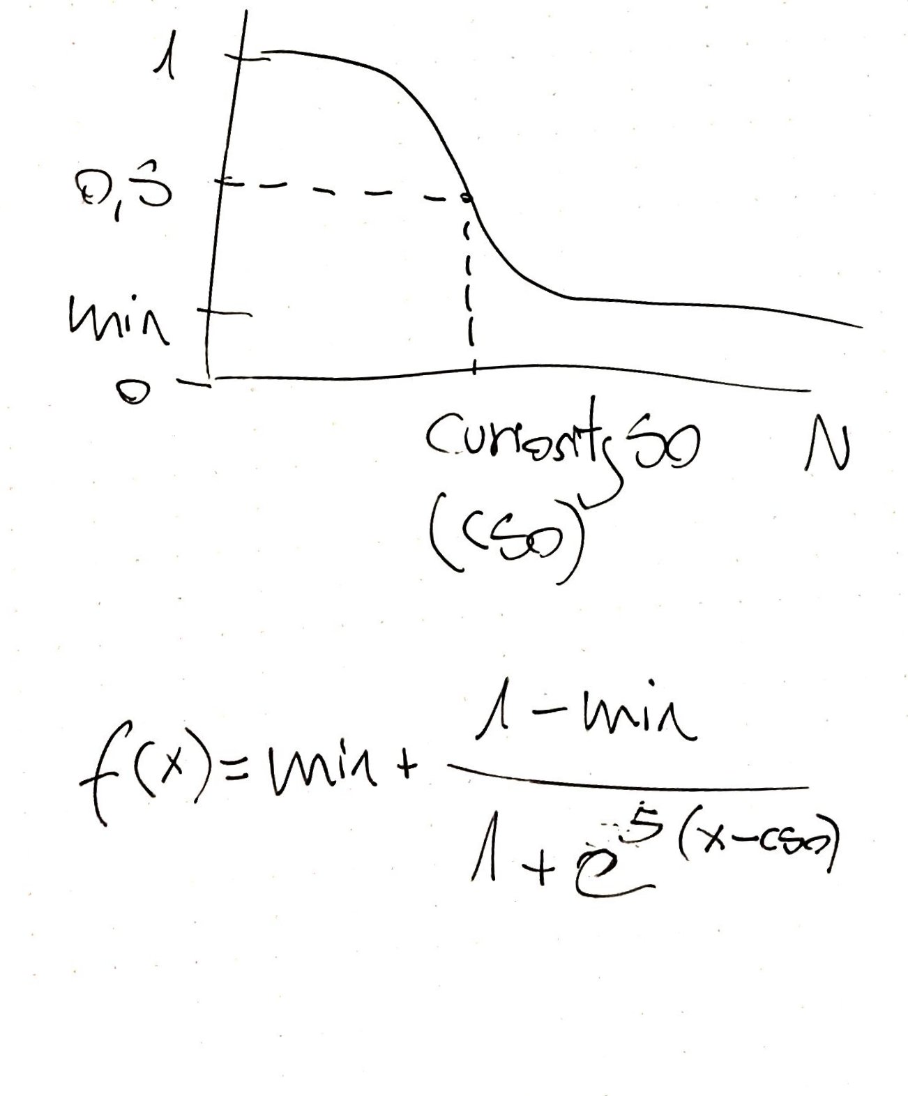
There are three hyper-parameters that can be adjusted (manually or iteratively):

Slope: It represents how fast the agent transitions from not trusting their experiences to trust them.

Curiosity50: It is the number of observations for a position that leads to a 50% chances of trusting the tree/library.

Min: It provides a basal level which is the percentage of random actions no matter how many observations the agent has for a certain position.

This type of learning curve allows the agent to adapt as it experiences the environment trusting more and more the past observations. Interestingly, the inclusion of a basal level would allow for the agent to adapt to a changing environment. This exploration/exploitation trade-off is well studied in the reinforcement learning field.

I have implemented the learning curve as a function in the script and set the default parameters as follows:

#Learning Curve

learn.curve <- function(x, min, slope, L50){
  min+((1-min)/(1+exp(-slope*(L50-x))))
}

min<-0.05
slope<-0.05
L50<-100

randomness <- learn.curve(1:250,min,slope,L50)
plot(randomness, type = "l", ylim = c(0,1), xlab = "Observations")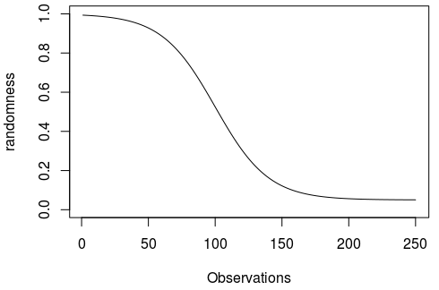

Finally, it is necessary to include a control parameter at the end of the action loop to overwrite the selected action with a random one according to the learning curve:

Curiosity <- learn.curve(experienceN,min,slope,L50)
    if(Curiosity > runif(1,min =0 , max= 1) ){
    action <- env_action_space_sample(server, instance_id)
    }

And that’s all!.
We have implemented a simple pure-algorithmic solution for the agent to learn.

To find the performance of the self-learner agent I have calculated the percentage of solved episodes as the number of episodes increase:

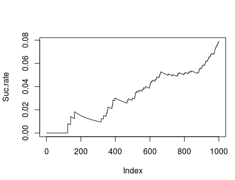
As you can see the agent starts to increase its performance just after running a few iterations.

Conclusions

After all these experiments it is possible to conclude that providing an agent with the possibility of having its own library of experiences improves the learning capabilities by increasing the flexibility.

In this post we have also seen that learning problems can be solved just by algorithms, no ML (at least how it is currently understood) is involved at all in this script.

Stay tuned for new AI solutions based in R.

---

Update 29th of January 2019

The ideas behind this post were purely based on my intuition about the optimal solutions to solve the environment; however, after reading more about RL I found out that my strategy to solve the environment could be considered a short of Q-learning strategy. Following posts will treat that topic with more detail