Introduction.

Few days ago I discovered the OpenAI Gym library which is a bunch of standardized AI environments written in Python to benchmark the skills of AI programs and scripts, aka agents.

All environments included in the OpenAI Gym library follow the deep reinforcement learning paradigm.

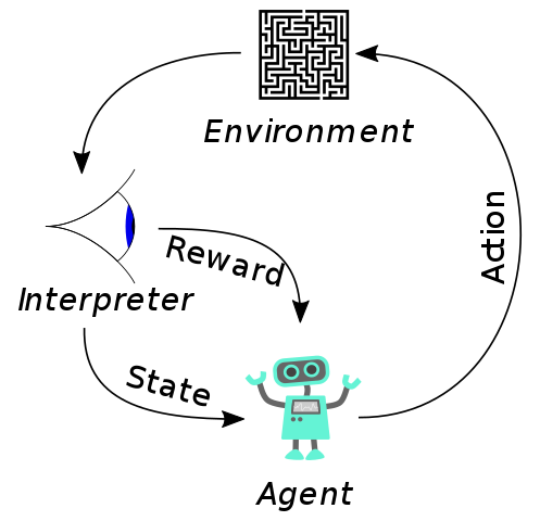
The agent observes the environment, makes a decision, performs an action, observes the how the environment has changed as a consequence of the action and gets a reward for that action. These processes are iteratively repeated until the episode is flagged as finished, solved or not.

The goal of this post is to introduce the very basics of OpenAI Gym in R and to generate the code of one simple agent as example. When it comes to deep reinforcement learning, R has been unfairly neglected in favor of Python; however, I would say that R and Python perform equally in 80% of machine learning-related tasks (especially since Keras, TensorFlow, MXNET etc… are accessible from R) and R definitely outperforms Python when deep statistical tasks are required.

Environment Installation.

The first thing that you have to do is to install OpenAI Gym, to do that you need to have Python and pip already installed in your computer so you can easily install the gym using pip:

pip install gym

Now you have all the environments installed in your computer; however, in order to access them from R you need to do a second trick. You need to install a web server that wraps the OpenAI Gym so we can reach it from R (or Matlab, or Julia, or C++…). This Gym http server is indeed a very interesting tool, not only because it allows you to play with the OpenAI Gym in non-python languages, but also because you could have one computer running the gym and the server while using other computers running the agents, parallelizing the test.
To install the server we need to run the following:

git clone https://github.com/openai/gym-http-api   
cd gym-http-api      
pip install -r requirements.txt         

Once you have the server installed you need to initialize it so you can access it from R:

nacho@Skadi:~$ python2.7 ./gym-http-api/gym_http_server.py

If everything went well you should get something like this:

Server starting at: http://127.0.0.1:5000           

Meaning that you have the server running in the localhost (127.0.0.1) listening on the port 5000 so any application or coding environment can access it, including those in other computers.

Finally, you will need to install the R package that wraps the functions required to access the Gym server as clients.

install.packages("gym")

Now you are ready to start with the coding.

Environment Initialization in R.

At the beginning of every script you will have to initialize the gym and an environment by running the following lines:

library (gym)
server <- create_GymClient("http://127.0.0.1:5000")

By this you assign the IP address and the port of the server to the variable server

env_id <- "CartPole-v0"

Here you assign the codename of the environment that you want to initialize to the variable env_id

instance_id <- env_create(server, env_id)

and finally you start the environment with codename env_id in the server located in our own computer (127.0.0.1:5000). The internal ID of the environment is assigned to instance_id which is a value that you will use during the rest of the script.

Available Environments.

OpenAI Gym offers dozens of challenges with different difficulty levels, including some Atari 2600 games and robotic tasks. Check the whole list here. Of all available enviroments CartPole is one of the simplest so it is a very convenient starting point.

CartPole.

CartPole is an environment consisting on a cart and a pole (surprise! surprise!)

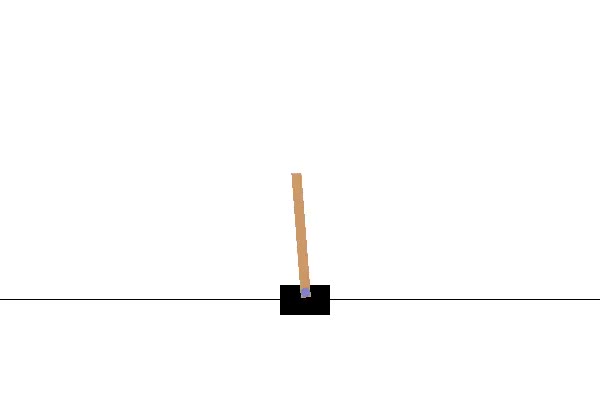
We control the cart by moving it to the right or the left so the pole, which is attached to the cart, pivots as a consequence. The goal of every agent that plays this environment is to maintain the pole in equilibrium preventing it to reach certain inclination.
As I mentioned before, all the environments included in the OpenAI Gym can take actions from the agent, providing observations and rewards.

Actions: In CartPole there are only two possible actions (1 and 0) that will move the cart to the left or the right.

Observations: At the beginning of the episode and after each action we obtain four observations corresponding to the cart position, the cart velocity, the pole angle and the pole speed at the tip.

Reward: In this environment we don’t get any reward based on our actions. However, since the goal is to maintain the pole in equilibrium as long as possible, the reward increases as the episode progresses. So the more steps the pole is in equilibrium the higher the reward. The environment is considered to be solved if the pole is in equilibrium for more than 195 timepoints.

Environment termination: An episode is considered to be a failure if the pole inclination is higher than 12 degrees or if the cart moves out of the screen.

Random policy.

In deep reinforcement learning a policy is defined as the list of internal rules encoded in the agent to execute one action based on the observations. The simplest policy that one can imagine is the random policy so the agent does not care about any observation and it just performs actions randomly.
Lets see how we encode this very simple policy:

  #dfEyes records: rewards, observations, status and actions
  dfEyes<-as.data.frame(t(rep(NA,4)))
  colnames(dfEyes)<-c("Obs1","Obs2","Obs3","Obs4")
  
  #The first thing we need to do is to reset the environment
  #we get the first 4 observations
  ob <- env_reset(server, instance_id)
  
  #Everything is recorded in dfEyes
  dfEyes[1,1:4]<-ob
  dfEyes$iteration[1]<-0
  dfEyes$Reward[1]<-NA
  dfEyes$Done[1]<-FALSE
  dfEyes$action[1]<-NA
  
  #Since the episode is considered to be solved after 195 steps
  #we establish the maximum number of steps in 200
  max_steps<-200
  for (j in 1:max_steps) {
   
  #The action is randomly sampled from all possible actions
  action <- env_action_space_sample(server, instance_id)
   
  #The results of the action are stored in results 
  #If render = TRUE the server will render the episode in a new window
  results <- env_step(server, instance_id, action, render = TRUE)
   
  #Everything is stored the dfEyes
  dfEyes[j+1,1:4]<-results[[1]]
  dfEyes$Reward[j+1]<-results[[2]]
  dfEyes$Done[j+1]<-results[[3]]
  dfEyes$action[j+1]<-action
  dfEyes$iteration[j+1]<-j
  dfEyes$round<-i
  
  #The episode stops if the termination conditions are reached
  if (results[["done"]]) break
  }
  

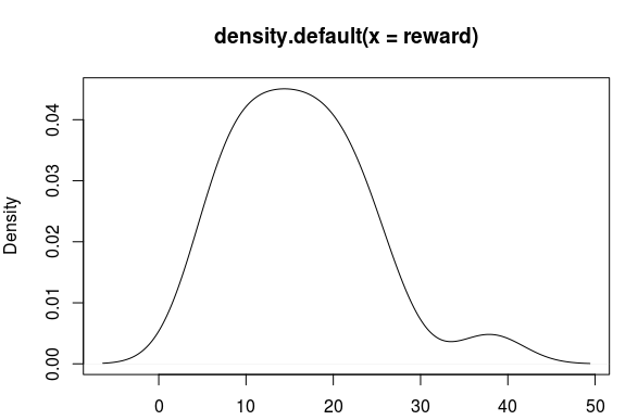
An agent executing this policy behaves like this:

It doesn’t look very effective with a median reward of 15.5 (n=200).

Decision Making Algorithms.

From previous results it is clear that we need to implement some kind of decision making algorithm in the agent in order to solve the CartPole environment.

It seems that the CartPole can be solved using a linear regression decision making algorithm, meaning that there exist Weight1, Weight2, Weight3, Weight4 and Bias such as the following formula solves the environment:

Action = Obs1·Weight1 + Obs2·Weight2 + Obs3·Weight3 + Obs4·Weight4 + Bias

However, in order to expand our algorithm to non-linear problems, we are going to implement an slightly more advance algorithm: the simplest possible neural network with 2 neurons connected by 10 weights, and we are going to perform a random search to find the 10 weights.

We will run episodes in batches (n=5) and we will stop the search once a batch gets an average reward >= 195. In more advanced scenarios in which complex networks are required or in those in which the space of valid weights is smaller, we will need to implement gradient descents and backpropagations, but in this case random search is more than enough to solve the CartPole environment as you will see.

Here is the scheme the basic neural network that we are going to implement:

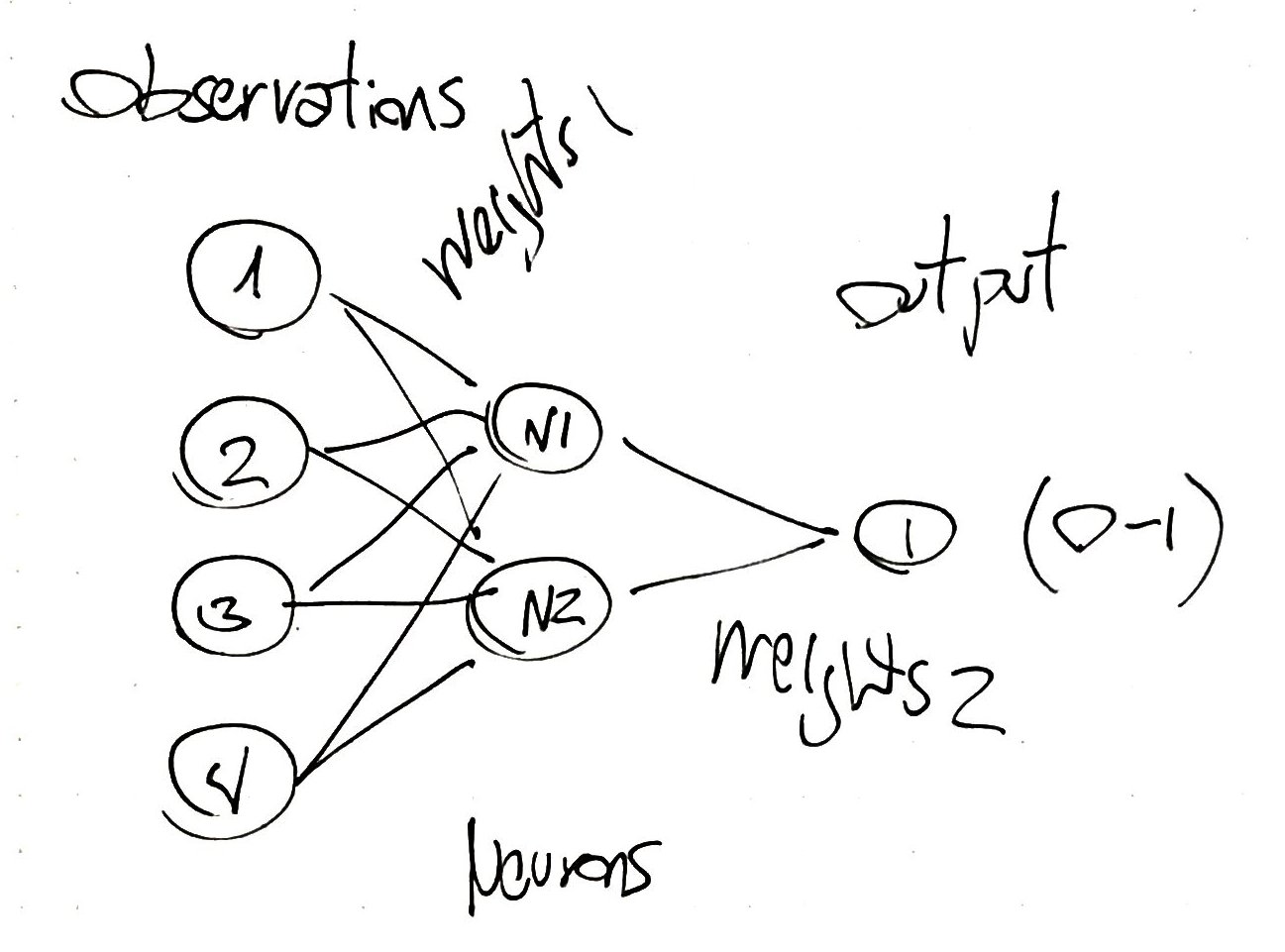
and here is the code ExplorationRandomSearchNN.R:

library(sigmoid)

Neurons <- 2
Observations <- 4
Neuron.layer<-rep(NA,Neurons)

#Random initialization of weights in a matrix and a vector
weightsN1 <-  matrix(data = runif(((Observations)*Neurons),
             min = -1, max = 1), ncol = Observations, nrow = Neurons)
weightsN2 <- rep(runif(Neurons,min = -1, max = 1), Neurons)

#Neurons values computation
for (i in 1:nrow(Input)) {
  for (h in 1:Neurons) {
  
Neuron.layer[h]<-sigmoid(sum(Input[i, 1:Observations]*weightsN1[h,]), method = "tanh")  
  }
Input$Out[i] <- round(sigmoid(sum(Neuron.layer*weightsN2),
                    method = "logistic"))
}

I have used tanh activation for the internal layer of neurons because I wanted to capture the negative signs of the observations without normalizing the data since it would be difficult to normalize the data from the observations (See Note1). For the output neuron I used the logistic function so the output falls in the 0-1 range.

Finally we put the neural network and the Gym together:

library(gym)
library(sigmoid)

server <- create_GymClient("http://127.0.0.1:5000")
 
#Create environment
env_id <- "CartPole-v0"
 
instance_id <- env_create(server, env_id)

iterations <- 5
reward <- 0
done <- FALSE
rounds<-50
Neurons <- 2
Observations <- 4
Neuron.layer<-rep(NA,Neurons)
max_steps<-200

for (k in 1:(rounds)) {

#dfGod is the dataframe where everything is stored
dfGod<-as.data.frame(t(c(1:9)))
dfGod<-dfGod[!1,]

#Random initialization of weights

weightsN1 <-  matrix(data = runif(((Observations)*Neurons),
                              min = -1, max = 1), ncol = Observations,
                              nrow = Neurons)

weightsN2 <- rep(runif(Neurons,min = -1, max = 1), Neurons)

for (i in 1:(iterations)) {
  dfEyes<-as.data.frame(t(rep(NA,4)))
  colnames(dfEyes)<-c("Obs1","Obs2","Obs3","Obs4")

  ob <- env_reset(server, instance_id)
  dfEyes[1,1:4] <- ob
  dfEyes$iteration[1] <- 0
  dfEyes$Reward[1] <- NA
  dfEyes$Done[1] <- FALSE
  dfEyes$action[1] <- NA
  
  for (j in 1:max_steps) {
  
Input<-dfEyes[j,1:Observations]

for (h in 1:Neurons) {

Neuron.layer[h]<-sigmoid(sum(Input[, 1:Observations]*weightsN1[h,]), method = "tanh")  
                                           
   }

action <- round(sigmoid(sum(Neuron.layer*weightsN2), method = "logistic"))
results <- env_step(server, instance_id, action, render = TRUE)

dfEyes[j+1,1:4] <- results[[1]]
dfEyes$Reward[j+1] <- results[[2]]
dfEyes$Done[j+1] <- results[[3]]
dfEyes$action[j+1] <- action
dfEyes$iteration[j+1] <- j
dfEyes$round <- i
t.zero<-unlist(ob)
                   
if (results[["done"]]) break

  }
  
dfEyes$Reward <- nrow(dfEyes)
colnames(dfGod) <- colnames(dfEyes)
dfGod[(nrow(dfGod)+1):(nrow(dfGod)+nrow(dfEyes)),] <- dfEyes
                                                       
}

dfGod<-dfGod[complete.cases(dfGod),]
Reward<-mean(unique(dfGod$Reward))

#If the mean of the reward is higher than 195 it is solved
if (Reward>=195) break

}

if (Reward>=195) print(paste("Solved after:", k,
                             "rounds", sep = " " ))
                             
#Closing the environment
env_close(server,instance_id)

The first time I run the script I got the following

[1] “Solved after: 3 rounds”

Conclusions.

In this post I have covered the very basics of deep reinforcement learning, the installation and setting up of the OpenAI Gym library and the creation of a simple but efficient AI agent able to solve the CartPole environment in few rounds. Moreover, this agent is flexible enough to solve other simple AI problems in which (1) the reward is established at the end of the episode and (2) the observation space is simple enough.

Notes.

Note1: The normalization could be done by using the minimum an maximum values described in the OpenAI Gym wiki, but in a real world scenario that information might be unknown and therefore impossible to normalize the data accurately.

Note2: The chain of actions that solves the problem is somehow expeceted: mainly 0s and 1s alternating.

*Note3: If you liked this post check my follow-up post:CartPole Under the Hood

dfGod$action
[1] 1 0 1 0 0 1 0 1 0 1 0 1 0 1 0 0 1 0 1 0 1 0 1 1 0 1 0 1 0 1

Bibliography and Sources of Inspiration.

[1] Deep Reinforcement Learning, Hands-on.
[2] Kevin Frans Blog.
[3] OpenAI Gym.
[4] Gym http Server.
[5] Gym Library in R