Introduction.

In my last post I was showed how to implement AI strategies to solve the CartPole environment, assigning and testing sets of 10 random values as weights of a very simple neural network. In this post, we are going to investigate a bit more on what is going on during these processes. In machine learning, weights are the internal parameters that are used to transform the observations into the predictions. The weights are usually initiated in a random manner and tuned during the training process so the predictions are more and more accurate. We could say that the training process is, indeed, the adjustment of the weights of the model.
In our neural network, we don’t tune them, we randomly assign values to the weights and check the performance of the agent; however, this strategy only works if the space of working-weights is big enough, so it is possible to find them just by chance.

Distribution of valid sets of weights.

In our model the chance of getting a model that works is so high that the first time that I run the model, I obtained a valid set of weights able to solve the environment just after 3 rounds. However, how likely is indeed to find a valid set of weights?
To answer this question I modified the script so it doesn’t stop when the environment is solved so it is possible to count the total number of valid models after several rounds.
After 1500 rounds I obtained the following distribution of successes:

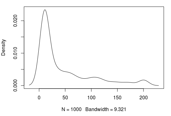
Around 3% of all combinations of weights are able to solve the environment. Nevertheless, as you can see from the plot, there is a large range of agents in terms of success, most of them don’t work at all, some of them perform better than a random set of weights and some of them solve the environment.

Neural network vs linear model.

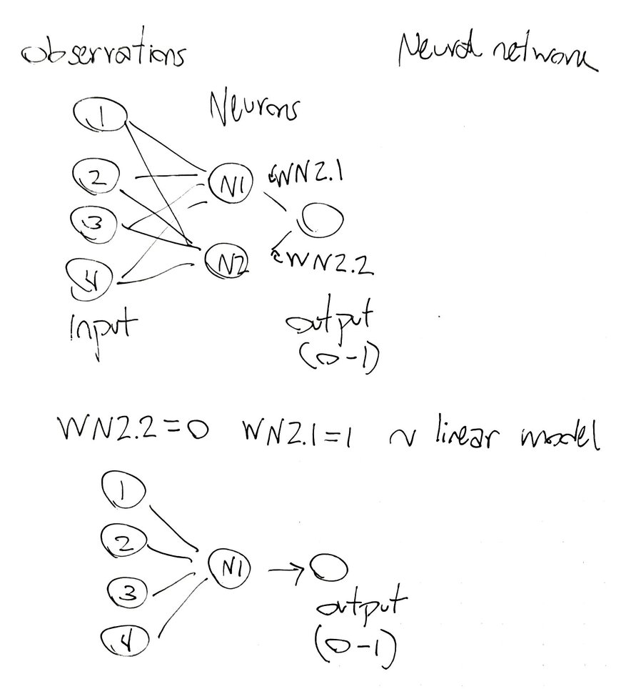
In the last post I already mentioned that the CartPole environment can be solved by finding the weights (and intercept) of a linear model like this:

Action = Obs1 * Weight1 + Obs2 * Weight2 + Obs3 * Weight3 + Obs4 * Weight4 + Intercept 

However, this type of linear models (without the intercept) is actually a special case of neural networks in which the weight connecting one neuron with the output (WN2.2) is 0 and the other weight of the other neuron is 1 (WN2.1):

So I explored the weights of the model, especially the distribution of WN2.2 and WN2.1 to see if the presence of linear regression models was somehow related with the ability of the agent to solve the CartPole:

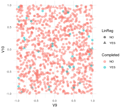
In this plot V9 represents the weight WN2.1 and V10 WN2.2. In blue are represented those WN2.1 and WN2.2 values that are able to solve the CartPole (together with the other 8 weights). The triangles represent those values of WN2.1 and WN2.2 in which our neural network approximates to a linear regression model (very high or low ratios between WN2.1 and WN2.2).

First of all, it seems that all the ranges of WN2.1 and WN2.2 are permitted for the agents able to solve the CartPole. It also seems that some of the solving agents (3 out of 39) have a linear regression policy. So the next question is if the NNet agents perform differently from the LinReg ones in any condition.

Neural networks seem to be more stable in noisy conditions.

Just from a visual inspection of the episodes executed by different agents, we can find that even though all of them solve the environment there are variations in their behavior.

LinReg-Agent-1

NNet-Agent-1

If you carefully look at how the pool balances, it becomes clear that the two agents act differently. That suggests that there might also exist differences in the performance of the different agents. Unfortunately, there is no easy way to run the CartPole for more than 200 steps without touching the Python code of the gym, so it would be difficult to find out how the different agents would perform in longer episodes. However, we could introduce a noise parameter to evaluate the performance of the agents in a noisy environment and compare them.
Noise, in this context, can be understood as a random modification of the observations that the agent perceives and I have implemented it as follows:

#Noise level up to 70%
Noise<-0.7
    for (l in 1:Observations) {
    dfEyes[j,l]<-dfEyes[j,l]+(runif(1, min = -Noise, max = Noise)*dfEyes[j,l]) 
    }
    Input<-dfEyes[j,1:Observations]

The agent senses the environment with a random distortion in all the observations up to a 70% of the real value (added or subtracted). We can think of this type of noise in a real-world situation in which the sensors connected to the agent are faulty or imprecise. This type of situations is actually very common in some delicate computer-assisted operations such as those carried out in the aerospace industry (you can read more about this here).

I re-evaluated the performance of the LinReg (n=3) and NNet (n=36) agents under these new noisy conditions and I found out that none of the LinReg agents was able to solve the environment; however, almost half of the NNet agents were still able to solve it:

LinReg agent #1 + Noise

NNet agent #5 + Noise

This suggests that neural network-based policies provide more stability to the agent than linear regressions ones. However, the number of observations is too low to conclude it without any doubt and more simulations and networks in which WeightN2.1 and WeightN2.2 are forced to 1 and 0 respectively are required to conclude that beyond any doubt.

Anyhow, it is clear that there are a lot of approaches from the different agents to solve the environment and that some of them are more resistant to noise interferences.

Artificial Generation of Agents Able to Solve the CartPole.

Since the weights are what define an agent, we could say that they represent “the software of the software” and the neural network architecture is the “hardware of the software”. Until this point, we have seen that the different agents loaded with different versions of the “software” perform distinctly; therefore, it would be very interesting to expand the number of agents so we could study and maybe rank them better.
In this section, I am going to show you an iterative approach able to generate thousands of agents in just a few steps.

The rationale behind this strategy is that it is logical to expect that all working sets of weights have something in common, meaning that there is an internal hidden relationship between the 10 weights that form a set that works, and this is the hypothesis that we are going to test. To do that we need to implement another deep neural network in which we are going to use the 10 weights as inputs and the ability to solve the CartPole as output to train the model.

For the deep neural network, we are going to use a standalone library that we can access from R: h2o and we are going to train the network using the 1500 sets of weights that we have already obtained.
I like h2o because it is simple but pretty flexible, you can implement deep neural networks, random forests, gradient boosting machines, linear regressions or model ensembles among others in few lines. It also has a function to perform hyperparameter searches, which makes it a very complete library for basic (and not that basic) machine learning tasks.

The goal of this post is not to talk about h2o, how to install it or how to run it but you can read about those topics here.

We are going to implemented a simple classifier using a basic deep neural net with two internal layers of 24 neurons (I was playing a little bit with the architectures and 24-24 performed fairly well).

 
#h2o initialization
h2o.init()

#Transforming the output variable into a binary columns with two factors
dfWeights$Completed[dfWeights$Completed=="YES"]<-1
dfWeights$Completed[dfWeights$Completed=="NO"]<-0
dfWeights$Completed<-as.factor(dfWeights$Completed)

#Split the dataset into training and testing to validate the performance
dfWeightsTrain<-dfWeights[1:900,]
dfWeightsTest<-dfWeights[901:1000,]

#Load the datasets into h2o
df.h2oTrain <- as.h2o(dfWeightsTrain)
df.h2oTest <- as.h2o(dfWeightsTest)

  NNet    <-         h2o.deeplearning(x= 1:10,  #Weights
                     y=11,  #completed column
                     stopping_metric="logloss",
                     distribution = "bernoulli",
                     loss = "CrossEntropy",
                     balance_classes = TRUE,
                     validation_frame = df.h2oTest,
                     training_frame	=	df.h2oTrain,
                     hidden = c(24,24),
                     nfolds = 5,
                     fold_assignment = "Modulo",
                     keep_cross_validation_predictions = TRUE,
                     epochs = 10) 

After the training step, I checked the performance of the model on the test set. It predicted two out of the three working agents and predicted as positive only one out of 100 non-working agents, so it is good enough for the purpose.

P<-h2o.predict(NNet, df.h2oTest)
dfWeightsTest$predicted<-as.vector(P$predict)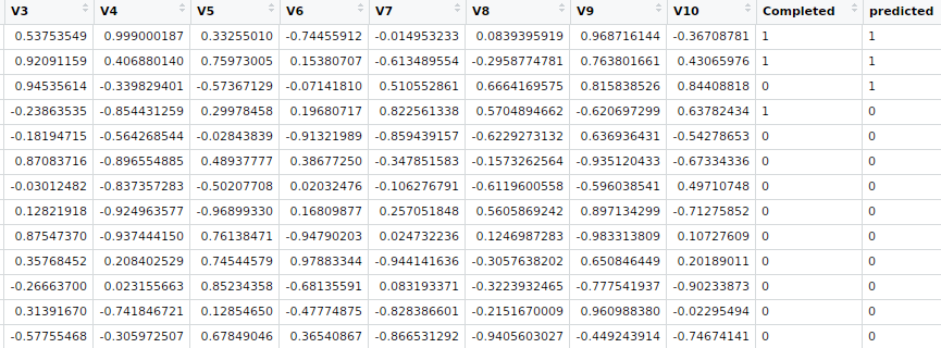

Next, we will create 1000 new agents by generating a matrix of random sets of weights:

weights.space <- as.data.frame(matrix(runif(10000, min = -1, max = 1), ncol = 10, nrow = 1000))
weights.space.h2o <- as.h2o(weights.space)

Then we re-trained the model merging the training and the testing sets and predict which agents in the matrix would solve the CartPole.

Agent.Pred<-h2o.predict(NNet, weights.space.h2o)
weights.space$predicted<-as.vector(Agent.Pred$predict)

The model predicts 108 out of 1000 agents to be working so let’s try them out in the gym environment:

#Restart the gym
instance_id <- env_create(server, env_id)
Agents<-subset(weights.space, weights.space$predicted == 1)

for (k in 1:nrow(Agents)) {
  weightsT<-Agents[k,1:10]
  
  #dfGod is the dataframe where all the observation for all iterations are stored
  dfGod<-as.data.frame(t(c(1:9)))
  dfGod<-dfGod[!1,]
  
  print(paste("Round",k,sep = " "))
  for (i in 1:(iterations)) {
    dfEyes<-as.data.frame(t(rep(NA,4)))
    colnames(dfEyes)<-c("Obs1","Obs2","Obs3","Obs4")
    
    ob <- env_reset(server, instance_id)
    dfEyes[1,1:4]<-ob
    dfEyes$iteration[1]<-0
    dfEyes$Reward[1]<-NA
    dfEyes$Done[1]<-FALSE
    dfEyes$action[1]<-NA
    
    for (j in 1:max_steps) {

      Input<-dfEyes[j,1:Observations]
      
      Neuron.layer[1]<-sigmoid(sum(Input[, 1:Observations]*weightsT[1:4]), method = "tanh")  
      Neuron.layer[2]<-sigmoid(sum(Input[, 1:Observations]*weightsT[5:8]), method = "tanh")
            
      action<-round(sigmoid(sum(Neuron.layer*weightsT[9:10]), method = "logistic"))
      results <- env_step(server, instance_id, action, render = TRUE)
      
      dfEyes[j+1,1:4]<-results[[1]]
      dfEyes$Reward[j+1]<-results[[2]]
      dfEyes$Done[j+1]<-results[[3]]
      dfEyes$action[j+1]<-action
      dfEyes$iteration[j+1]<-j
      dfEyes$round<-i
      t.zero<-unlist(ob)
      
      if (results[["done"]]) break
    }
    dfEyes$Reward<-nrow(dfEyes)
    colnames(dfGod)<-colnames(dfEyes)
    dfGod[(nrow(dfGod)+1):(nrow(dfGod)+nrow(dfEyes)),]<-dfEyes
  }
  
  dfGod<-dfGod[complete.cases(dfGod),]
  Reward<-mean(unique(dfGod$Reward))
  RewardT[k]<-Reward

  print(Reward)
}

#Closing the environment
env_close(server,instance_id)

The performance is not as good as in training set since only 24 out of the 108 agents were able to solve the environment; however, the good thing about our strategy is that we can use the newly created agents to improve the performance of the h2o model by merging the old set of weights with the new ones that are already tested and iteratively retrain the model again and again.

After doing this several times we will end up with a highly improved model, check out the code here.

Update 02.January.2018

After few hours of running the script I found two things:

1. The script preferentially finds LinReg agents:
   

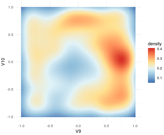
In the 2D density plot of working weights(WN2.1 and WN2.2) it is possible to observe an enrichment in LinReg agents (WN2.1=1 and WN2.1=1). A possible explanation for this is that is it the occurrence of a combination of working weights follows, complex rules that can’t be fully identified by our current model.

2.The script doesn’t improve the identification of working agents as quickly as I expected. After 50 rounds of training only 33% of the predicted working-agents are really working. Because of this two observations I decided to implement a more advance h2o model in which the hyperparameters (the settings of the model) are iteratively searched:

dfWeights$Completed<-as.factor(dfWeights$Completed)
df.h2oWeights<-as.h2o(dfWeights)

df.split <- h2o.splitFrame(data=df.h2oWeights, ratios=0.90)
df.train <- df.split[[1]]
df.test <- df.split[[2]]

#Hyperparameter search (architecture,epochs, act function, drop-out)
hyper_params.NN <- list(
  hidden=list(c(32,32,32),c(64,64), c(80,40,20), c(40,40), c(20,20), c(12,12,12)),
  input_dropout_ratio=c(0,0.05, 0.1),
  rate = c(0, 0.1, 0.005, 0.001),
  rate_annealing=c(1e-8,1e-7,1e-6),
  epochs = c(5, 10, 20),
  l1 = c(0, 0.00001, 0.0001), 
  l2 = c(0, 0.00001, 0.0001),
  rho = c(0.9, 0.95, 0.99, 0.999),
  epsilon = c(1e-10, 1e-8, 1e-6, 1e-4),
  activation = c("Rectifier", "Maxout", "Tanh", "RectifierWithDropout", "MaxoutWithDropout", "TanhWithDropout")
  )

#Search criteria (it will explore 100 models)
search_crit.NN<-list(strategy = "RandomDiscrete", max_models = 50)

grid.NN <- h2o.grid(
  x=1:10, 
  y=11,
  algorithm="deeplearning",
  nfolds = nfolds,
  fold_assignment = "Modulo",
  keep_cross_validation_predictions = TRUE,
  seed = 1,
  grid_id="dl_grid.NN", 
  training_frame=df.h2oWeights,
  balance_classes=TRUE,
  distribution="bernoulli",
  #adaptive_rate=T,                
  loss="CrossEntropy",
  stopping_metric="logloss",
  #max_w2=10,                      
  hyper_params=hyper_params.NN,
  search_criteria = search_crit.NN
)

#Order the models by their accuracy
grids.nn<- h2o.getGrid(grid_id = "dl_grid.NN",
                       sort_by = "accuracy",
                       decreasing = TRUE)
grids.nn

After 150 models the maximum accuracy acchieved was 0.804 (architecture 32-32-32, l1/l2=0). This suggests that even though we have achieved a significant enrichment, some of the combinations that lead into working-agents might just be unpredictable by a neural network and other ML strategies such as GBM or random-forests might improve the prediction.

Conclusions.

In this example I have shown how to implement a very simple classifier but imagine the possibilities. For example, one could apply a scoring system based on the performance in noisy environments to train and retrain the model and obtain a perfect set of agents:

“The best thing about being me, there’s so many “me”s”
Agent Smith (The Matrix Reloaded, 2003)

As you can see there is endless fun under the hood of AI implementations and the more control you have over your algorithms and functions the deeper you can explore.

Notes.

Note 1: First I tried to fit the relationship between weights and the ability to solve the CartPole using a linear regression model but the performance was terrible, implying that the relationships are non-linear.

Note 2: When I say h2o is used for basic machine learning task I am talking about a task that does not require advance modifications of the model. However, h2o is used in many production environments in which the basic analyses are enough.