
Creating VAEs in R (Part 1)
Introduction.
Of all machine-learning models, I personally find autoencoders (AE) really fascinating. AE are a special type of unsupervised models assembled by two sub-models: an encoder and a decoder. Encoder and decoder have an inverted shape and between them there is an internal layer which is the layer with fewer dimensions of the model and after training it will contain the latent space of the input.
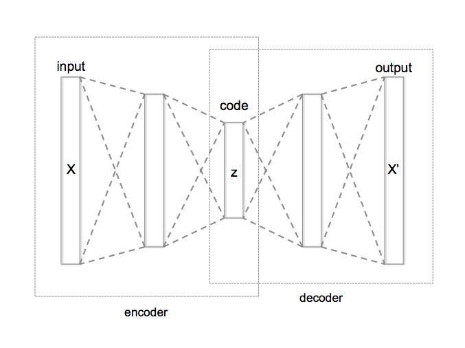 The latent space is a hidden and simplified representation of the data in which more similar elements lay closer.
Alternatively to the typical supervised models, AE are not trained to generate a dependent variable, they are trained so the original data is regenerated after passing through the model. This special way of training a model gives the autoencoders their most relevant characteristic: the generation of the latent space. Due to this capability, AE can be used to reduce the dimensionality of the data, to filter out the noise in the data, to find anomalies and, what I think is more interesting, to generate new data through the so-called variational autoencoders (VAE).
VAE can learn the hidden characteristics of any given data and use that knowledge (stored in the latent space) to generate novel data. For example, we can train a VAE with thousands of pictures of human faces and the model will generate new pictures of faces just by sampling the latent space learned from the training data.
VAE and music generation.
On the internet, there are many posts and literature about VAEs generating faces, hand-written digits or pictures of cats; however, the use of VAEs to generate music is less commonly found and this is what I will try to implement in this series of posts. In this first post I will describe an attempt to generate a novel national anthem based on 135 anthems.
Before constructing any model, it is possible to anticipate that the task will be very difficult just for one reason: the sample size. We have only 135 samples; however, machine learning models usually require several thousands of samples during the training process. So if you are reading the post expecting an amazing result I have to disappoint you, there won’t be any new anthem in the end… But who cares, “the journey is the destination”.
Data format and data loading.
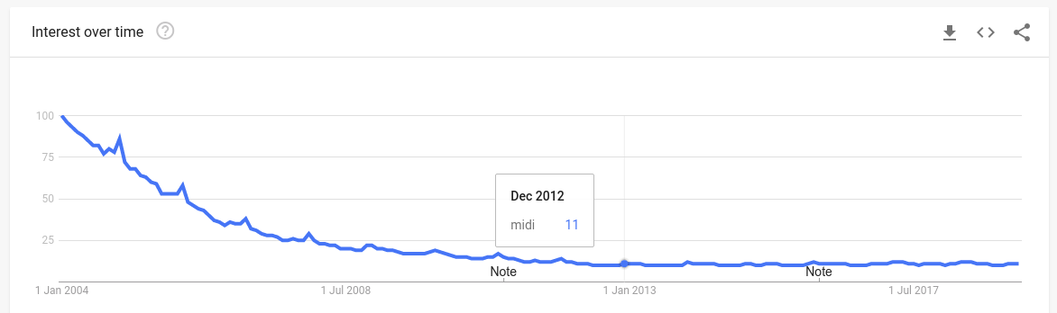
For this project, I am going to use MIDI files which basically encode the score of a musical piece. Because of their small size, MIDI files were very popular at the beginning of the internet when the bandwidth was so low that transferring a single .mp3 file could take 15-30 minutes; however, nowadays they are only used by musicians in some contexts, so the popularity of the format has dropped and not even the common internet browsers can reproduce it.
There is a lot of information encoded in a MIDI file which is interpreted by MIDI player to know how to reproduce the music. The most interesting parameters are the global time, which is the time when the different events occur, the events, which are the notes to play (encoded as numbers from 1 to 128), the duration of the event referred to the global time, the channel which is the instrument executing those events and the track which usually correspond to the instrument; although, it is possible to find several tracks per channel (e.g. channel: Piano, track1: left-hand, track2: right-hand).
The first thing that we have to do is to extract all those parameters and tweak them into a ML friendly format, something not as trivial as it might look at a first glance.
You can download all the MIDI files used in this post here.
To load the files into R I am going to use the package TuneR which is a very useful library to work with audio files.
library(tuneR)

#Data loading
path<-"/home/nacho/Downloads/Midi/NationalAnthems/"
files<-list.files(path)
setwd(path)

df<-list()
pb <- txtProgressBar(min = 1, max = length(files), initial = 1)
for (i in 1:length(files)) {
  setTxtProgressBar(pb,i)
  read<-readMidi(files[i])
  df[[i]]<-getMidiNotes(read)
}
This part of the code stores all the filenames into the file variable and then it loads the anthems one by one into a list (df). I have used two functions of the TuneR library, readMidi and getMidiNotes. readMidi produces a raw file that it is tranformed into a more friendly format using the getMidiNotes function to produce something like this:
     time length track channel note notename velocity
1       0   1186     2       0   63      d#'       97
2    1196    241     2       0   62       d'       91
3    1442    223     2       0   63      d#'      109
Next, I decided the format of the data. Although the optimal format it is the one that looks like a pianola roll (x= time, y= note, z= channel), accommodating the 135 anthems would require a huge and very sparse array of 135 by 100.000 by 128 by 12 which would require several Gb just to fit it into memory. Unfortunately, I don’t have enough RAM (I currently have only 4Gb and it would require at least 16Gb).
Pianola roll plot for the Brunei national anthem.
I needed to find a less sparse way to represent the data in order to feed the model and I decided to go for a format based on the output of getMidiNotes: by constructing an array with 4 dimensions.
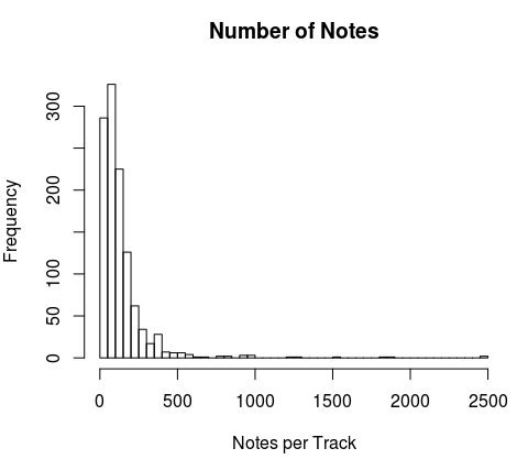
df.array <- array(data=0, dim=c(length(df),Notes.N,3, channels))The first dimension contains the different anthems; the second the number of notes; the third one the notes, the duration of the note and the starting time for that note; finally, the last dimension contains the different tracks. The size of the second dimension was decided based on the histogram of the number of notes per track per anthem:
#Check maximum number of elements per track
t4<-0
for (i in 1:length(df)){
  tracks<-unique(df[[i]]$track)
  for (j in 1:length(tracks)) {
  t4 <- c(t4, length(df[[i]]$time[df[[i]]$track==tracks[j]]))
  }

}
t4<-t4[-1]
hist(t4, breaks=60, main="Number of Notes", xlab="Notes per Track")

Notes.N<-150
You probably have the same feeling about it that I had: “it is not going to work because it is way too artificial (especially the third dimension)”. Additionally, the duration of the note is not exactly the same as the figure represented in the score. During this project, I learned that a trick used by the MIDI format to be able to represent the same figure when it is played two consecutive times in the score is to slightly cut the length of the first one in order to create the small silence to distinguish the two pulses. All that leads to another problem, the quantization of the file. We can think in quantization as the granularity of the file, making two identical figures to have different length in different files with different quantization. Unfortunately, I checked and not all the files were quantized equally, so the same note with the same duration has different values in two different files.
With all this said I was pretty sure that the model wouldn’t work, but I continue with it because again, the goal is the journey not the destination and who knows, it is possible that the model could capture the patterns and the non-linearities of the scores, it is impossible to know until we try.
Here is the code to fill in the array:
#Array filling
for (i in 1:length(df)) {
  tracks<-unique(df[[i]]$track)
  for (j in 1:min(length(tracks),channels)) {

  dummy.note<-df[[i]]$note[df[[i]]$track==tracks[j]]
  #+1 to make starting time at 1
  dummy.time<-df[[i]]$time[df[[i]]$track==tracks[j]]+1
  dummy.length<-df[[i]]$length[df[[i]]$track==tracks[j]]

  df.array[i,1:min(length(dummy.note),Notes.N),1,j]<-
  dummy.note[1:min(length(dummy.note),Notes.N)]

  df.array[i,1:min(length(dummy.length),Notes.N),2,j]<-
  dummy.length[1:min(length(dummy.length),Notes.N)]

  df.array[i,1:min(length(dummy.time),Notes.N),3,j]<-
  dummy.time[1:min(length(dummy.time),Notes.N)]
  }
}
The channels, notes and times are padded with 0s. Note that there are whole channels padded with zeroes in some anthems.
Once the array is ready, we need to define the model. In this post, I am going to use Keras and I am going to use the VAE described in the Rstudio webpage devoted to Keras as a starting point:
Parameters for tuning:
#Parameters
epsilon_std <- 1.0
filters <- 36
latent_dim <- 2
intermediate_dim <- 256
batch_size <- 10
epoch <- 100
and the model:
#### Model
dimensions<-dim(df.array)
dimensions<-dimensions[-1]

Input <- layer_input(shape = dimensions)

Notes<- Input %>%
  layer_conv_2d(filters=filters, kernel_size=c(5,1), activation='relu',
  padding='same',strides=1,data_format='channels_last')%>%
  layer_conv_2d(filters=filters*2, kernel_size=c(5,1), activation='relu',
  padding='same',strides=1,data_format='channels_last')%>%
  layer_conv_2d(filters=filters*4, kernel_size=c(5,3), activation='relu',
  padding='same',strides=1,data_format='channels_last')%>%
  layer_conv_2d(filters=filters*8, kernel_size=c(5,3), activation='relu',
  padding='same',strides=1,data_format='channels_last')%>%
  layer_flatten()
This part of the model tries to find patterns in the input by using convolutions; the first two layers try to find patterns in a 5x1 way, that means that it tries to find patterns in five consecutive events in for each sub-dimension (note, length and time). The other two layers combine all dimensions to find patterns that might be relating them.
Next, there are several fully-connected layers with 256, 256/2 and 256/4 units connecting the 72000 values coming from the flattering of the convolutions. The a 2D latent space is created.
hidden <-
Notes %>%
layer_dense(units = intermediate_dim, activation = "sigmoid") %>%
layer_dense(units = round(intermediate_dim/2), activation = "sigmoid") %>%
layer_dense(units = round(intermediate_dim/4), activation = "sigmoid")

z_mean <- hidden %>% layer_dense( units = latent_dim)
z_log_var <- hidden %>% layer_dense( units = latent_dim)
Then, the sampling function from the latent space is created.
sampling <- function(args) {
  z_mean <- args[, 1:(latent_dim)]
  z_log_var <- args[, (latent_dim + 1):(2 * latent_dim)]

  epsilon <- k_random_normal(
    shape = c(k_shape(z_mean)[[1]]),
    mean = 0.,
    stddev = epsilon_std
  )
  z_mean + k_exp(z_log_var) * epsilon
}

z <- layer_concatenate(list(z_mean, z_log_var)) %>%
      layer_lambda(sampling)
Next, the decoder.
output_shape <- c(10, dimensions)

Output<- z %>%
  layer_dense( units = round(intermediate_dim/4), activation = "sigmoid") %>%
  layer_dense( units = round(intermediate_dim/2), activation = "sigmoid") %>%
  layer_dense(units = intermediate_dim, activation = "sigmoid") %>%
  layer_dense(units = prod(150,3,filters*8), activation = "relu") %>%
  layer_reshape(target_shape = c(150,3,filters*8)) %>%
  layer_conv_2d_transpose(filters=filters*8, kernel_size=c(5,3), activation='relu',
  padding='same',strides=1,data_format='channels_last')%>%
  layer_conv_2d_transpose(filters=filters*4, kernel_size=c(5,3), activation='relu',
  padding='same',strides=1,data_format='channels_last')%>%
  layer_conv_2d_transpose(filters=filters*2, kernel_size=c(5,1), activation='relu',
  padding='same',strides=1,data_format='channels_last')%>%
  layer_conv_2d_transpose(filters=9, kernel_size=c(5,1), activation='relu',
  padding='same',strides=1,data_format='channels_last')
Now we can create the model:
vae <- keras_model(Input, Output)To compile the model we need a loss function and in the case of VAE, we define a custom loss function containing two elements:
- The difference between the input and the output, to be sure that the model recreates the input as accurate as possible. We can achieve that by minimizing the mean square logarithmic error (MSLE) between input and output.
- The difference between elements in the latent space to aggregate them around the center of the latent space (0,0). The reason for this is to prevent gaps between different groups of elements because the model wouldn’t know how to interpret those empty regions of the latent space, generating aberrant outputs. Again, keep in mind that in our case we only have an element (anthem) per group (country). This regularization parameter can be written as a Kullback-Leibler divergence (KL) term to be minimized.
Note that I have used MSLE instead MSE because the values to approximate are produced by a RELU function (which can produce any value larger than zero as output) and not normalized, that makes the first term of loss function using MSE way higher than the KL so the KL would be misrepresented during the training. Additionally, I have included two parameters to fine tune the weight of both terms inside the loss function so it would be possible to use MSE by setting a very small Loss_factor.
Reg_factor <- 0.5
Loss_factor<-1

# Custom loss function
vae_loss <- function(x, x_decoded_mean_squash) {

  x <- k_flatten(x)
  x_decoded_mean_squash <- k_flatten(x_decoded_mean_squash)

  xent_loss <- Loss_factor*loss_mean_squared_logarithmic_error(x, x_decoded_mean_squash)
  kl_loss <- -Reg_factor*k_mean(1+z_log_var-k_square(z_mean)-k_exp(z_log_var), axis =-1L)

  k_mean(xent_loss + kl_loss)
}
Now we can compile the model, create the training and test sets and train the model to see what happens…
vae %>% compile(optimizer = "rmsprop", loss = vae_loss)
summary(vae) #For inspection

val<- sample(dim(df.array)[1], 10)
xval<- df.array[val,,,]
xtrain<-df.array[-val,,,]

reset_states(vae) #To test different models

date<-as.character(date())
logs<-gsub(" ","_",date)
logs<-gsub(":",".",logs)
logs<-paste("logs/",logs,sep = "")

history<-vae %>% fit(x= xtrain,
                     y=xtrain,
                     batch_size=batch_size,
                     epoch=epoch,
                     validation_data = list(xval, xval),
                     callbacks = callback_tensorboard(logs),
                     view_metrics=FALSE,
                     shuffle=TRUE)

tensorboard(logs)
Note that I have created a unique identifier to be able to track every experiment in the tensorboard without mixing them up.
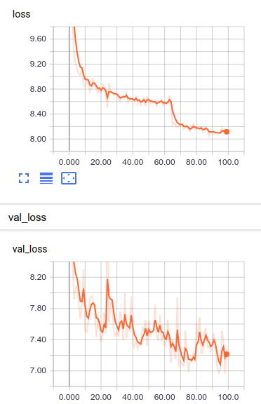
Validation
Based on the training curves it seems that the training went ok; however, the only way to fully appreciate the performance of the model is to try to reconstruct one of the anthems and see how similar is to the original one. In this case we are going to recreate the first anthem (Afghanistan).
 #Regeneration of sample #1
  Samp1.gen <- predict(vae, array(df.array[1,,,],
  dim = c(1,150,3,9)), batch_size = 10)

      Samp1.gen[1,,1,] <- round(Samp1.gen[1,,1,])
      Samp1.gen[1,,2,] <- round(Samp1.gen[1,,2,])
      Samp1.gen[1,,3,] <- round(Samp1.gen[1,,3,])

      to.plot <- as.data.frame(Samp1.gen[1,,,1])
      colnames(to.plot) <- c("Note", "Length", "Time")
      to.plot$Channel<-1

      for (i in 2:9) {
        dummy <- as.data.frame(Samp1.gen[1,,,i])
        colnames(dummy) <- c("Note", "Length", "Time")
        dummy$Channel<-i
        to.plot<-rbind(to.plot,dummy)
      }

  ggplot(to.plot)+
    geom_line(aes(x=Time,y=Note, colour=as.character(Channel)))+
    theme_minimal()
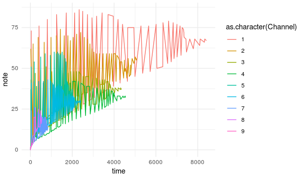
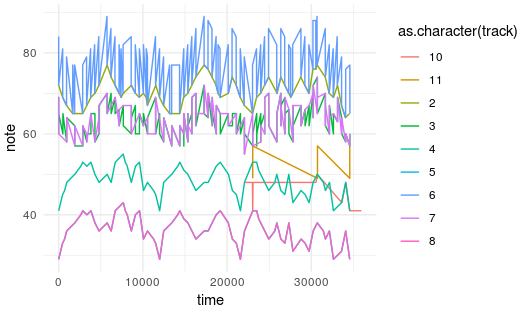
The recreation of the anthem looks very different from the original:
ggplot(df[[1]])+
  geom_line(aes(x=time,y=note, colour=as.character(track)))+
  theme_minimal()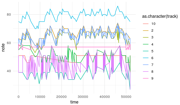
All that means that our model couldn’t find any hidden pattern common to all anthems or more precisely to the way I represented the anthems and any further investigation of the model such as data generation or inferecences from the latent space are useless.
So at this time I decided not to continue tuning the model but to change the input, using a more simple dataset with a higher number of examples.
Conclusions.
In this post we have seen what is a VAE and how to implement it in R. We have also seen how important is to choose a proper way to represent the data, wrong representations will make impossible for any model to learn any pattern at all. However, there are many tips in the post that might be useful, such as how to create a custom loss function, the use of Relu functions in the output to try to approximate non-normalized data or some coding tricks.
I hope you are not dissapointed by the negative results described in this post because at end…
“…Negative results are just what I want. They’re just as valuable to me as positive results. I can never find the thing that does the job best until I find the ones that don’t.”
Thomas A. Edison
Stay tune to find out how to create music using VAE in R. ;)

As always you can inspect the code described in this post here.