
It’s never aliens (Until it is)
Introduction.
“Are we alone in the universe?”.
When it comes to answering one of the most relevant questions that humanity has still open, we have to admit that we don’t have a clue.
The first historical references to the question are found in ancient Greece. Greek and Roman philosophers reasoned that since the universe seemed to be so vast, it would be reasonable to think that other “tribes” would be living somewhere out there. Later on, religious thinking displaced logical reasoning and humanity became special just because it was God’s will for humans to be special. It was not until the Renascent, when others started to ask the same question again: “If the Earth is no the center of the universe and there are other planets and stars, why should be life on Earth special?”
If you think for a second about the implications that answering that question would have, you soon realize how crucial it is for us, humans, to find the answer. It doesn’t matter the answer itself, just knowing with 100% certainty that there is (or that there is not) life somewhere else in the universe, would change our view of the universe.
Unfortunately, neither ancient greeks nor guys like Copernicus and Huygens had the technology to answer the question, and indeed we still don’t know if we can answer that question today. But here in this post, I will show you some of the current approaches that we, humans, are using to try to answer the question.

The Fermi paradox and the Drake’s equation.
In 1961 Frank Drake tried to shed some light on the mystery by turning the philosophical question into a parametric hypothesis. He estimated numerically the probability for another intelligent civilization to live in the Milky Way. For the first time in history, someone had tried to answer the question from a numerical point of view. According to Drake, we should be sharing our galaxy with another 10 intelligent civilizations with the ability to communicate. Is that too much? is that too little? Well… for sure we would not be able to detect our presence from 10K light-years (3,1kpc) which accounts for approximately 1/10 of the galactic size. Moreover, we would not be able to detect even the presence of Earth since the closest exoplantet detected is around around 6.5K light-years from us.
But coming back to Drake’s equations. It takes into account the following parameters:

R∗ = Rate of star formation
fp = Ratio of stars having planets
ne = Ratio of planets in the habitable zone of the stars
fl = Ratio of nethat would actually develop life
fi = Ratio of fl that would develop intelligent life
fc = Ratio of civilizations that develop a technology detectable from other planets
L = Time for which civilizations send detectable signatures to space
Of course, some of the parameters are purely theoretical; for instance, we don’t know how easy it is for a form of life to exist or to become intelligent. There is, indeed, a recent study in which the authors develop a theoretical Bayesian framework to estimate some of Drake’s parameters. In this paper, they argue that considering how early life arrived on Earth and how late this life became intelligent, acquisition of intelligence might not be an easy leap to make. However, the universe is vast, so big that even events with very low probabilities are likely to happen somewhere. Here is where Fermi’s paradox kicks in: If it is so likely that there is intelligent life somewhere in the observable universe, why haven’t we heard from them??!!
There are so many possible answers to try to solve the paradox that it would be impossible to mention them all, and still, it is a paradox because none of the arguments is strong enough to solve it. Maybe aliens are not interested in communicating, maybe they are too advanced for us to understand them, maybe there are “technological filters” like nuclear wars, climate changes, etc… wiping out civilizations once they reach these technological stages.
Again, we don’t know.
The SETI/Breakthrough programs
Since we haven’t been able to disprove any hypothesis regarding extraterrestrial intelligence so far, we can only keep scanning the sky looking for a signature of an intelligent civilization and this is what the SETI does. Through different initiatives, SETI scans most of the electromagnetic spectrum (from radio waves to light sources) trying to find non-natural signatures. However, the amount of data gathered so far is insanely big, that big that a comprehensive analysis using “humans” to analyze it would take a lot of years. We need machines to do the job.

SETI, through the Breakthrough program, has released massive datasets containing data from the closest 100000 stars. The data comes from The Parkes Observatory, The Green Bank Telescope and the Automated Planted Finder( Lick Observatory) and you can download everything here. The idea behind releasing such a dataset is to make it available for the community, so everyone can explore it and this is what I will do in this post: To establish a computational framework so that everyone can explore this and other astronomical datasets.
Navigating the data.
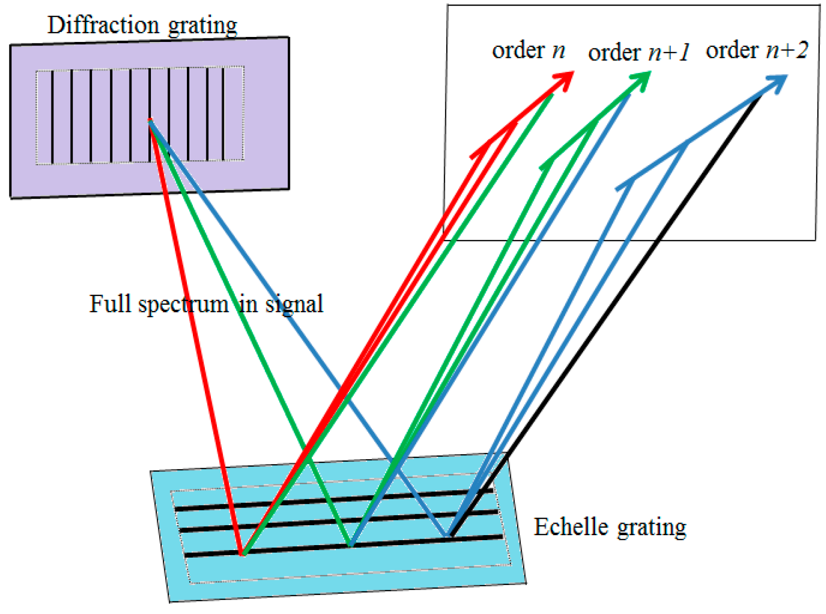
In this post, I will just focus on the APF dataset because of its simplicity. The APF dataset is a set of images in FITS format. Each image corresponds to the observation of one star at one particular time point. The “images” are indeed spectrograms that are generated by a telescope coupled with an echelle spectrograph that splits the light coming from a star into its different wavelengths. This allows us to measure the number of photons of each wavelength coming from that particular star: Here is an scheeme of an echelle spectograph:
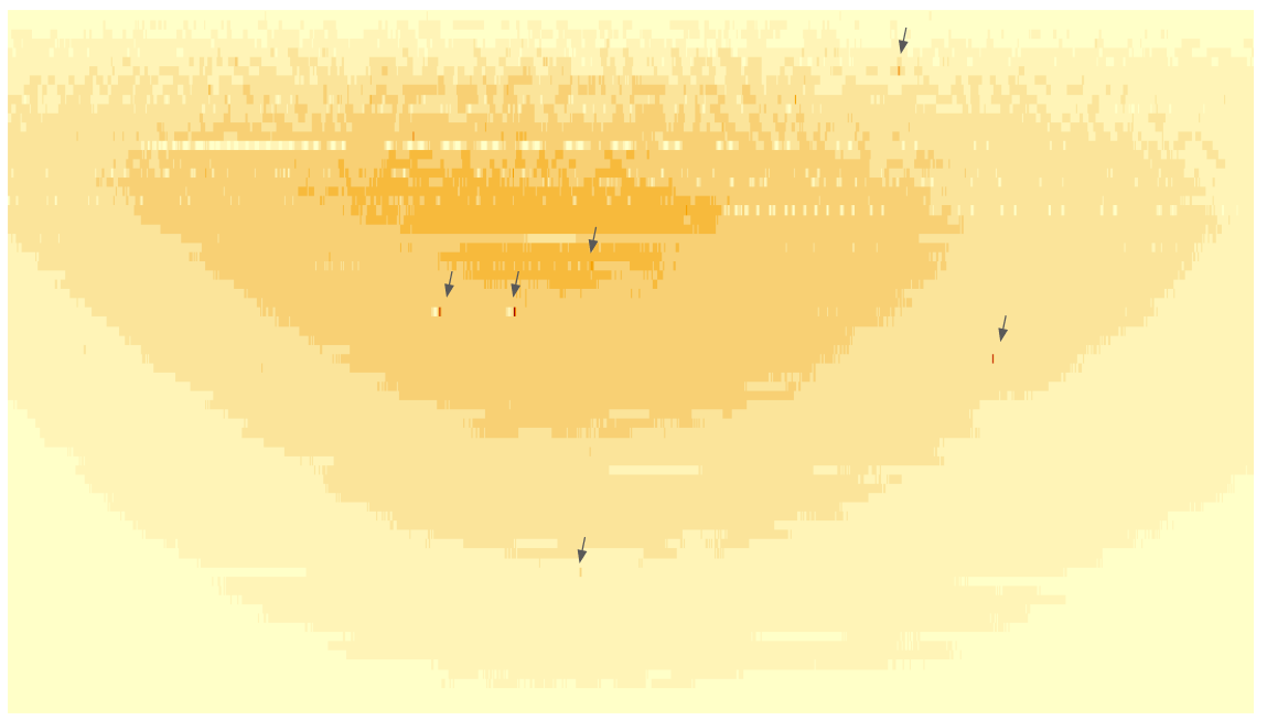
The raw images that we obtain from the echelle telescope look like this:
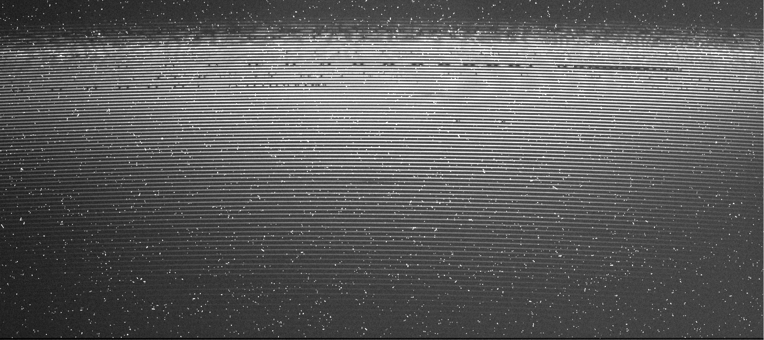
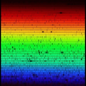
The image represents the diffraction of the light of a star. The wavelength increases from up to low and from left to right, so the photons with the lower wavelength (red) hit the top left corner and in the lower-left corner shows the number of photons with the highest wavelength (blue). If we assign a colour to each region we would have something like this:
As you can see, there are two features in the image: the shadows and the “tracks”. This is more obvious if we zoom in into the image:
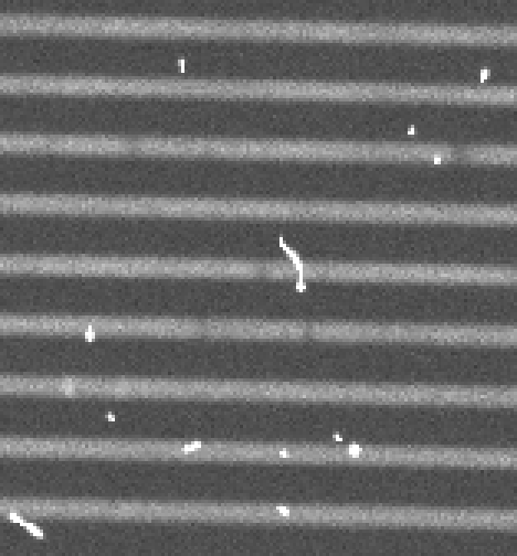
This pattern is indeed an artifact of the technique, not all the area on the image is covered by the diffracted light. We are interested only in the tracks of light because they are the ones that contain the information. Those “tracks” are called orders and we need a way to extract the information laying on the orders in a process called compression (basically because the resulting image with the important information is much smaller in size).
The first step in the compression is to find out where the tracks lay in the image.
The way to do it is a bit convoluted: We need to find functions that “draw” lines going through all the pixels of every track.
As you can see in the image, the tacks are curved and although this is normal in echelle spectra, it is a bit problematic for us because the functions that draw such curves are 4rd order polynomial functions like this one:
Now we only need a way to find a, b, c and d for each one of the 79 orders. I guess that different tools have their own algorithms but I had to develop my own to estimate the 5 parameters.
My algorithm finds the orders by identifying the tracks in the central region of the image, which is where all the tracks are better defined, and then, it goes track by track finding the parameters that satisfy the following two conditions:
- The curve must go through the point of the track identified in the central region that I call the anchoring point
- The mean of the pixels of the image that the function overlays must be maximized (meaning that we are avoiding the shades between tracks)
So let’s start coding it:
But before doing any of this, we need to load the FITS files and this is done in R using the FITSio library (We also load the rest of the libraries that we are going to use later on)
library(FITSio)
library(doParallel)
library(parallel)
library(foreach)
library(data.table)
library(ggplot2)
library(ggpubr)
library(ggrepel)
library(RCurl)

df<-readFITS("/home/nacho/SETI/ucb-bek230.fits")
df.img<-df$imDat
You can download the ucb-beck230.fits file from here. Now the image is stored in the df.img matrix with dimensions [2080,4608]. Although you can plot the image I don’t recommend it, the rendering is very slow and it is going to be difficult to see anything anyway. This is the best I have obtained by tweaking the zlim of the image function:
image(df.img, zlim = c(median(df.img)/2, median(df.img)*2))
As I said, the rendering is so inefficient that it even creates horizontal white stripes:
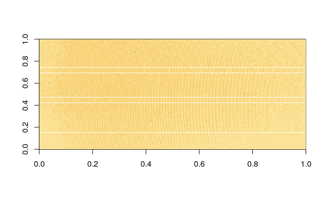
Next, we need to remove the background on the image and we do it by subtracting the value corresponding to the first 30 rows of the image, that never have a track:
baseline<-median(df.img[1:30,])
df.img<-df.img-baseline
Then, we look for the 79 peaks of photons corresponding to the orders at the center of the image:
#Identification of N peaks
df.img<-df.img-baseline
anchor.band<-round(ncol(df.img)/2)
track.width <- 10
track.n<-79
central.band<- df.img[,anchor.band]
#Remove cosmic ray
central.band[which(central.band>2500)]<-0

anchor.point <- vector()
for (i in 1:track.n) {
  anchor.point.dummy <- which(central.band==max(central.band))[1]
  central.band[(anchor.point.dummy-track.width): (anchor.point.dummy+track.width)]<-0
  anchor.point<-c(anchor.point, anchor.point.dummy)
}
anchor.point<-unique(anchor.point)
In this algorithm, the peaks are stored in the anchor.point vector.
This is how the order look like when they cross the central part of the image:
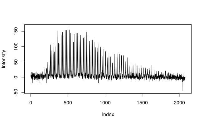
and this is how the algorithm finds the peaks:

Now that we have identified the orders in the central part of the spectrogram, we need to find the tracks. Note that the algorithm has some problems identifying lowest and highest orders (the signal in those wavelengths is so weak that the algorithm fails to detect them over the background noise).
As I mentioned above, we want to find those 4rd order functions that overlap the tracks. Since the function to be maximized is not differentiable, we will find the parameters by doing a random search. Parameters b, c, d, and e will take random values on a small range (because of the similar shape of the curves), so it will be easier for the model to find the optimal solution after a few iterations, let’s say 10000. The optimal solution is the one in which the mean of the values of the image defined by the functions is maximized.
Parameter a will be assigned to the only possible value that makes the curve going through the pixel identified on the central region. Since the algorithm has to find the parameters for each one of the 79 orders, it is possible to parallelize the code, so each processor gets the task of finding the parameters for one order. Here is the code to do it:
fitter <- function(x, a, b, c, d, e){
  y<-a + b*x + c*x^2 + d*x^3+ e*x^4
  return(round(y))
}

iterations<-10000

cores<-detectCores()-1
cluster.cores<-makeCluster(cores)
registerDoParallel(cluster.cores)

output<-foreach(i=1:length(anchor.point), .verbose = TRUE) %dopar%{
  #Function to call equation

#for (i in 1:length(anchor.point)) {

  x<-round(ncol(df.img)/2)
  y<-anchor.point[i]
  for (k in 1:iterations) {

  #Parameter generation
  b <-runif(1, min = -0.08, max= 0)
  c <-runif(1, min = 0, max= 1.6e-05)
  d <-runif(1, min = -1.1e-09, max= 1.5e-09)
  e<- runif(1, min=-1e-13,max= 2e-13)
  a<- y - b*x - c*x^2 - d*x^3 - e*x^4

  #call function
  row.ids<-fitter(c(1:ncol(df.img)),a,b,c,d,e)

  row.ids<-row.ids[row.ids>0]
  row.ids<-row.ids[row.ids<nrow(df.img)]

  if(length(row.ids)>100){
  indexes<-vector()
  for (j in 1:length(row.ids)) indexes[j]<-((2080)*(j-1))+row.ids[j]

  #Create evaluation metric
  score<-mean(df.img[indexes])

  if(!exists("best.score")) {
    best.score<-score
    best.params <- c(a,b,c,d,e,i)
    }

  if(score>best.score){
    best.score<-score
    best.params<-c(a,b,c,d,e,i)
    } }
  }
  return(best.params)
  rm(best.params)
  rm(best.score)
}

stopCluster(cluster.cores)

params.opt<-output[[1]]
for (i in 2:length(output)) {
  params.opt<-rbind(params.opt, output[[i]])

}
Now, we have found where the orders lay in the image and we need to extract their values. To do that, we average the value of the width of the track (approximately five pixels).
#Order extraction
for (i in 1:length(anchor.point)) {
  df.coord<-  as.data.frame(fitter(c(1:ncol(df.img)),a,b,c,d,e))
  colnames(df.coord)<-"Y"
  df.coord$X<-c(1:ncol(df.img))
  dummy.row<-vector()

  for (j in 1:nrow(df.coord)) {
    dummy.row[j]<-mean(df.img[c((df.coord$Y[j]-2):(df.coord$Y[j]+2)),df.coord$X[j]])
  }
  if(!exists("compressed")){
  compressed<-dummy
  }else{
  compressed<-rbind(compressed,dummy)
  }
}
Although this method works, the random nature of the parameters would make the extractions incomparable unless we align them using some common spectral features (eg. The H-band due to the hydrogen and/or iodine bands used to calibrate echelle spectrographs). If you find this algorithmic approach interesting, you can just take the code and develop it further but these additional tests and validations go beyond the scope of this post. Luckily for us, we don’t need to do the entire process for each spectrogram. We can just download the compressed spectrogram from the SETI webpage.
Scrapping SETI
Now that we have plan A (to download the compressed spectrogram) and plan B (to compress the raw spectrogram when it is needed), we can proceed downloading the data from the breakthrough database. To do that, we would use an index of the database which you can download here. This is the code to get information about the compressed files (reduced==TRUE) stored in the database.
files<-read.csv("/home/nacho/SETI/apf_log.txt", sep = " ", header = FALSE)
files<-files[-1,]
files<-files[,1:8]
files$reduced<-gsub(".*\\/r", "TRUE", files$V1)
files$reduced<-gsub("TRUE.*", "TRUE", files$reduced)
files<-files[files$reduced=="TRUE", ]

stars<- unique(as.character(files$V3))
stars.n<-vector()
for (i in 1:length(stars)) {
  stars.n[i]<-nrow(files[files$V3==as.character(stars[i]),])

}
stars<-stars[order(stars.n, decreasing = TRUE)]
stars.n<-stars.n[order(stars.n, decreasing = TRUE)]
This code extracts the information about the stars that are in the database and the number of observations for each one of them.
From there you could find information about your favorite star.
In this post, I’ll use KIC 8462852 as an example. To do that, I just need to find and download the files in the database that correspond to observations of KIC 8462852 (aka Tabby’s):
tabby <- files[grep("8462852", files$V3),]

tabby$link<-gsub("gs:\\/", "https:\\/\\/storage.googleapis.com", tabby$V1)
tabby$filename<-gsub(".*\\/","",tabby$V1)

for (i in 1:nrow(tabby)) {
  download.file(tabby$link[i], paste("/home/nacho/SETI/Tabby/",tabby$filename[i],sep = ""))
}
So, what’s the deal with KIC 8462852? KIC 8462852 is also known as Tabby’s star. Tabby’s is a star that became very famous a few years ago when it was found that it had abnormal reductions in the light intensity that were not consistent with any known stellar event. Several hypotheses were proposed to explain these unusual observations and one of them is the presence of a gigantic megastructure wrapping the star developed by a very advanced alien civilization to extract the energy of the star. Of course, once the alien hypothesis reached the media, the idea propagated exponentially.
Although the mystery is still unsolved, no radio emissions from Tabby’s have been detected and the most likely hypothesis nowadays is that the fluctuations could be originated by a cloud of asteroids/comets/dust there is still a strong interest in this star by the media, so let’s join the ufologist and explore Tabby looking for aliens.
Now that we have all the compressed spectra from Tabby’s in the same folder, we can load them into a 3D array in which the first dimension will be the temporal one.
# Load files directory Taby
files<-list.files("/home/nacho/SETI/Tabby/")

image.array<-array(data = NA, dim = c(length(files), 4608, 79))
date<-vector()
for (i in 1:length(files)) {
  dummy<-readFITS(paste("/home/nacho/SETI/Tabby/", files[i], sep = ""))
  date[i]<-dummy$header[25]
  image.array[i,,]<-dummy$imDat
}

wl<-readFITS("/home/nacho/SETI/apf_wav.fits")
wl<-wl$imDat
You might have noticed that the scripts use an additional file apf_wav.fits. That file is required to link the wavelength and the coordinates on the matrix.
Next, we normalize the data:
#Normalization
photons_norm<-vector()
for (timeevents in 1:dim(image.array)[1]) {
  photons_norm[timeevents]<-sum(image.array[timeevents,,])

}
photons_norm<-photons_norm/min(photons_norm)

for (timeevents in 1:dim(image.array)[1]) {
  image.array[timeevents,,]<-image.array[timeevents,,,drop=FALSE]/photons_norm[timeevents]

}
Finding artificial signatures.
Now that we have the data ready, we need a strategy to find the interesting stuff. How does an intelligent signature look like? We don’t really know, indeed, if someone on the closest star were looking at the Sun using an echelle telescope they could find biosignatures (if they were lucky enough to observe an eclipse and their telescopes were sensitive enough) but they would not be able to find any sign of intelligence in our solar system. They might find that the Earth’s atmosphere contains compounds difficult to explain by natural sources; however, we are not emitting anything strong enough on any visible wavelength to be detected. Of the two light anomalies that we could find using an echelle telescope (reduction or emission of photons), I find emissions much more interesting because they are more difficult to be explained by natural sources.
Why would a civilization want to emit any light beacon strong enough to be detected? We don’t know and we can’t even guess it but there’re fewer natural events emitting light on discrete wavelengths than those absorbing it.
One of the main sources of “contamination” on echelle spectrograms are cosmic rays, they appear as peaks of photons at any wavelength. To remove them, we will use statistical approaches. First, we are going to generate 3 arrays, one for the mean, one for the median, and one for the standard deviation at every time point for all the wavelengths (represented as the values of the array):
#Spike finder
mean.array<-matrix(data = NA, nrow = dim(image.array)[2], ncol = dim(image.array)[3])
sd.array<-matrix(data = NA, nrow = dim(image.array)[2], ncol = dim(image.array)[3])
median.array<-matrix(data = NA, nrow = dim(image.array)[2], ncol = dim(image.array)[3])
for (i in 1:dim(mean.array)[2]) {
mean.array[,i]<-apply(image.array[,,i], 2, mean)
sd.array[,i]<-apply(image.array[,,i], 2, sd)
median.array[,i]<-apply(image.array[,,i], 2, median)
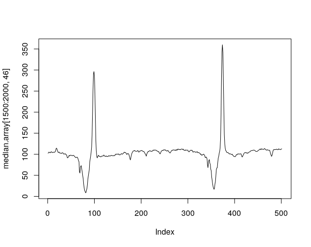
}By plotting a wavelength range, we can see how this approach cleans the spectrogram from cosmic rays. Let’s look at the Hydrogen-alpha absorption line of Tabby’s (coordinates on the arrays [1500:2500,54]). The Hydrogen-alpha absorption line is a region of the spectrogram where there are fewer photons than in surrounding areas because of the absorption due to the star’s own hydrogen.

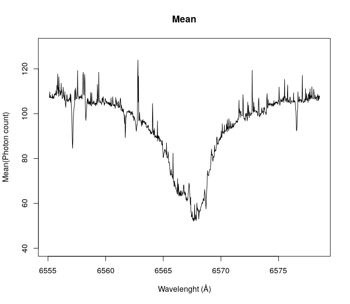
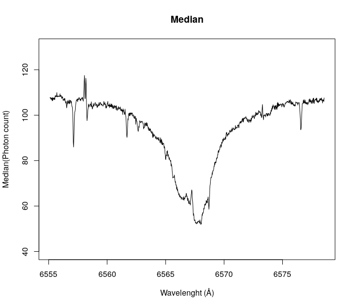
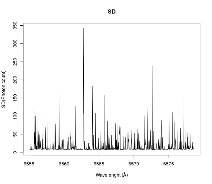
As you can see the median gets rid of most of the noise on the observations, so we will continue using this array. It is possible to find anomalies just by visual inspection (later we will find a programmatic way to find them).
Let’s first start with the series of two peaks and two valleys in the center of the image.
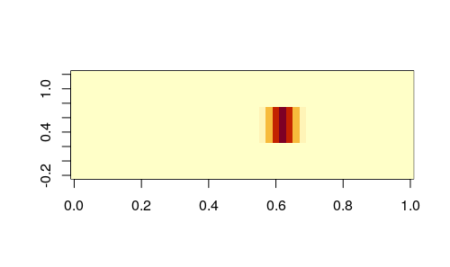
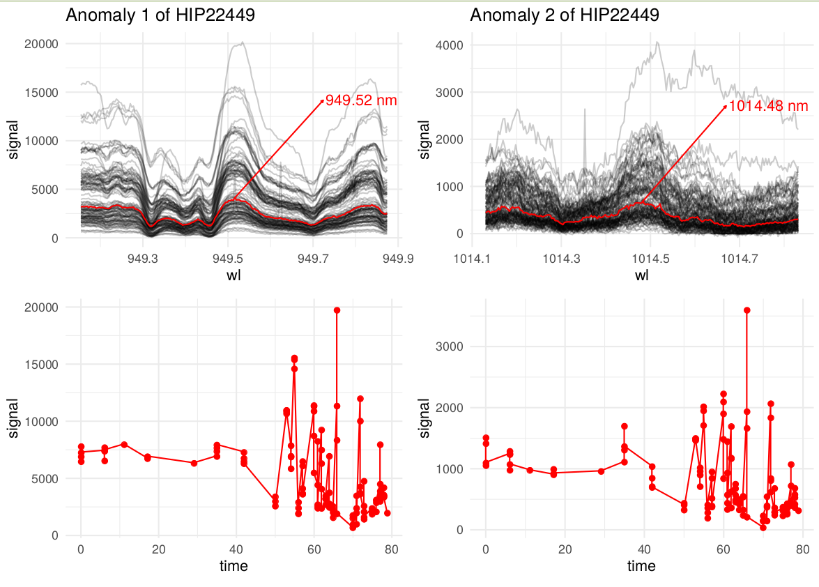
This is the profile:
and this the overlay of all observations
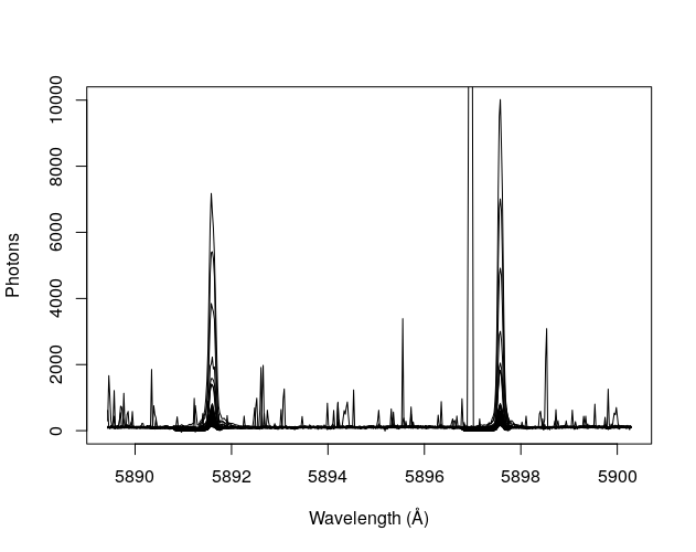
If we plot their intensity over the time-series this is how it looks:
The two peaks overlap almost perfectly, which means that whatever source it is, it must cause both.
So those are the features of the misterious signal.
- It causes two peaks with maxima around 5891.623Å and 5896.737Å.
- The peaks are alongside two valleys.
- Same source.
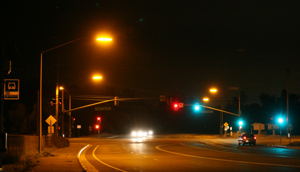
And the solution is that these peaks actually are caused by the sodium vapor lamps of the cities nearby. When the astronomers talk about the luminic contamination they are really serious about it.
Now we can try to solve the other mysterious peaks
The emission at 5578Å has this profile, what that is… we don’t know, but at least we have a human signature to compare with, the sodium vapor lamps, if the profile is similar we infer that the source of both peaks is the same: humans
Although the correlation is not perfect, the three maxima correlate, suggesting that the source is probably related to human light sources as well
Problem partially solved, let’s chase no ghost here!
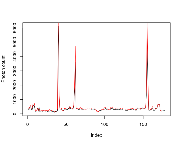
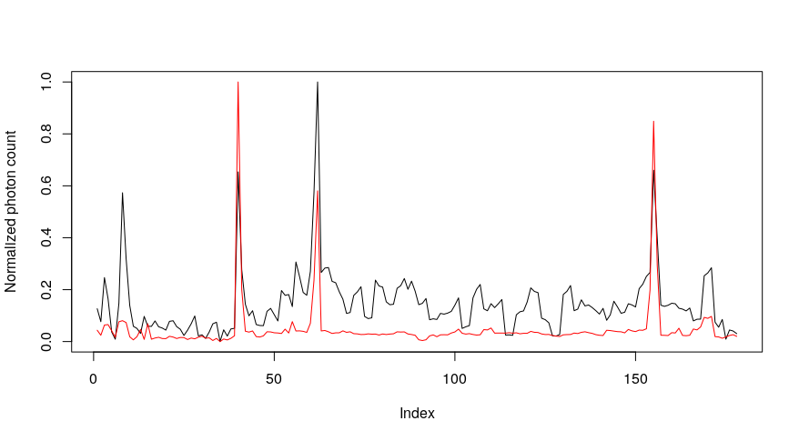
Next one: Peak at 6302.073Å
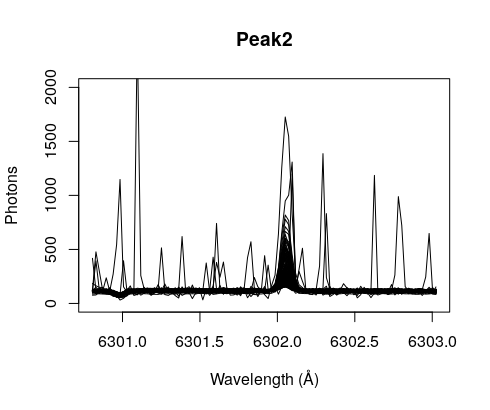
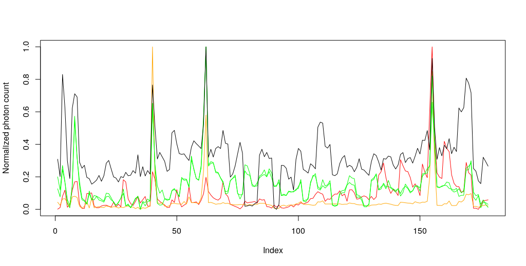
If we plot together the 3 peaks we get this (the red line is the peak at 6302.073Å)
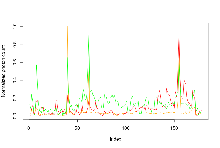
Again, they partially overlap, suggesting at least a common origin for some of the peaks. Whether this common origin is we don’t know, maybe it is related to the weather or the time of the day when the observations were taken.
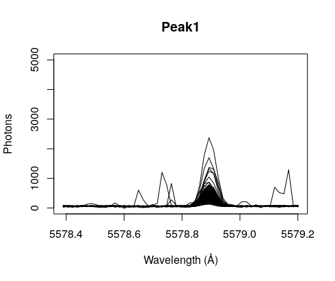
Next peak: 5578.931Å
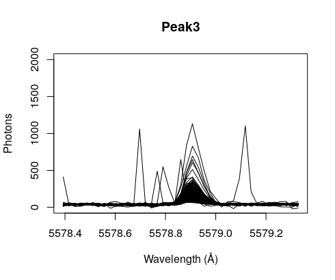
Let’s plot all the peaks together.
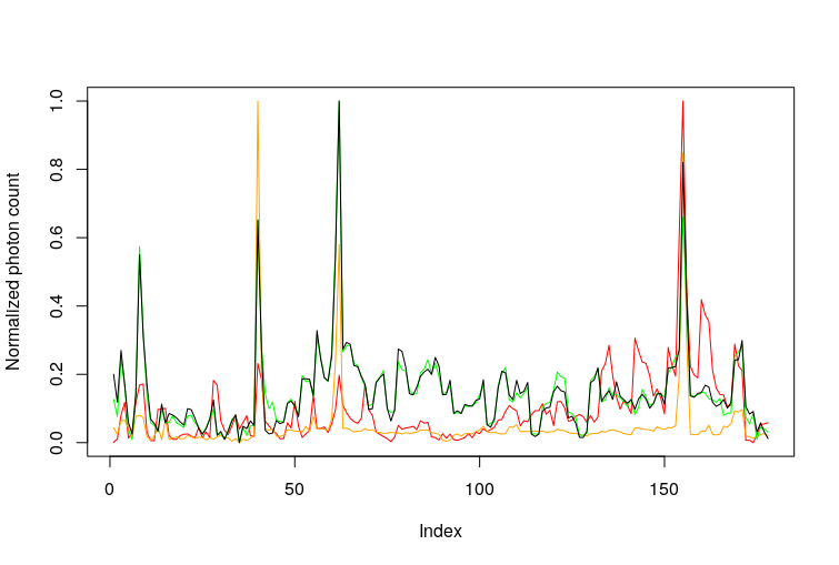
It seems that the green one and this (black) have an almost perfect correlation (as in the case of the sodium vapor lamps). Of course, it is indeed the same peak that appears in two orders of the spectrogram with wavelengths estimated at 5578.931Å and 5578.909Å. As you can see in this plot, it is possible to find overlapping wavelengths on the order 41 and 42:
Let’t look at the last peak: 9383.27Å This one falls on the infrared range of the spectra and it looks like this.
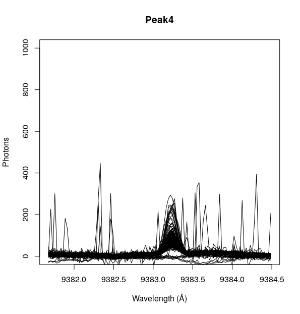
Sadly, the high-intensity peaks overlap with the other non-natural peaks, which means no alien lasers on Tabby’s thrusting solar sails.
Automatizing the analysis.
As you can imagine, analyzing this way all the spectra for all stars in the database would require an enormous amount of time. However, it is possible to do this programmatically. This script can connect to the database, get one star at a time, and run the analyses to identify all the peaks and also to run the correlations between peaks. The peaks are ranked by their signal-to-noise rate so if the ones with the lowest index are the interesting ones.
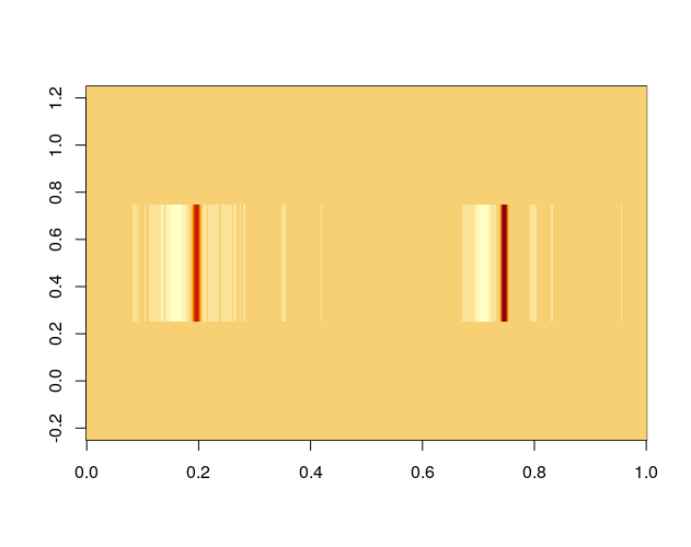
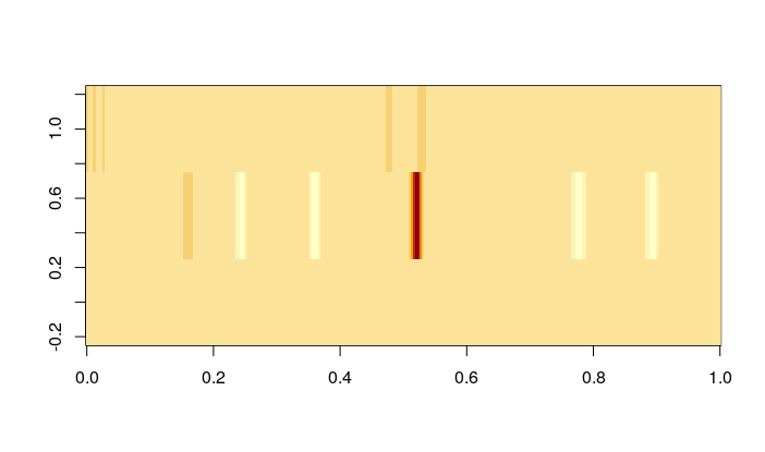
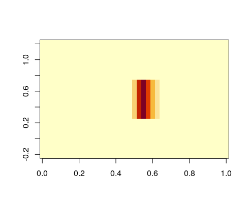
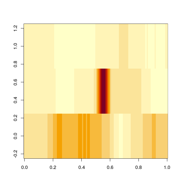
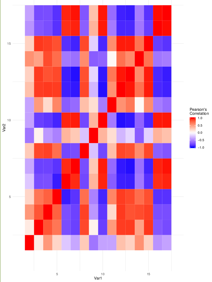
This is an example of the output of my aline-scapping tool: It generates a plot like this one:
A correlation matrix.
And the profile of the spectrum binned, so it is possible to visualize it.
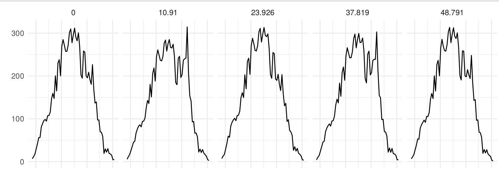
Additionally, it saves the results of the peaks and surrounding areas as csv.
Do you like it? Would you like to explore the data without spending the days that the analysis requires? No problem. I have uploaded the results of a lot of them here, so you can just surf them looking for alien signatures.
Where to go from here.
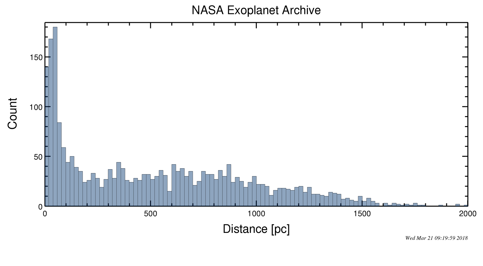
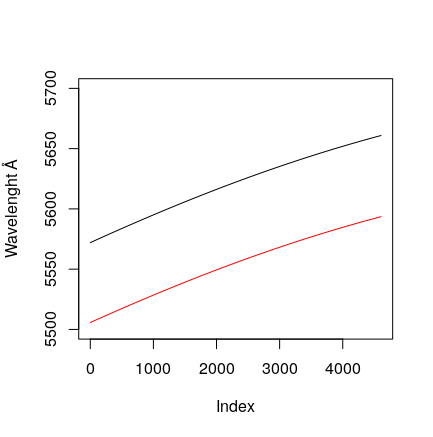
If you liked this post and you wanted to do something similar, you can apply what I used here including the scrapping method. You could start finding correlations between the two filters of the Gaia telescope…
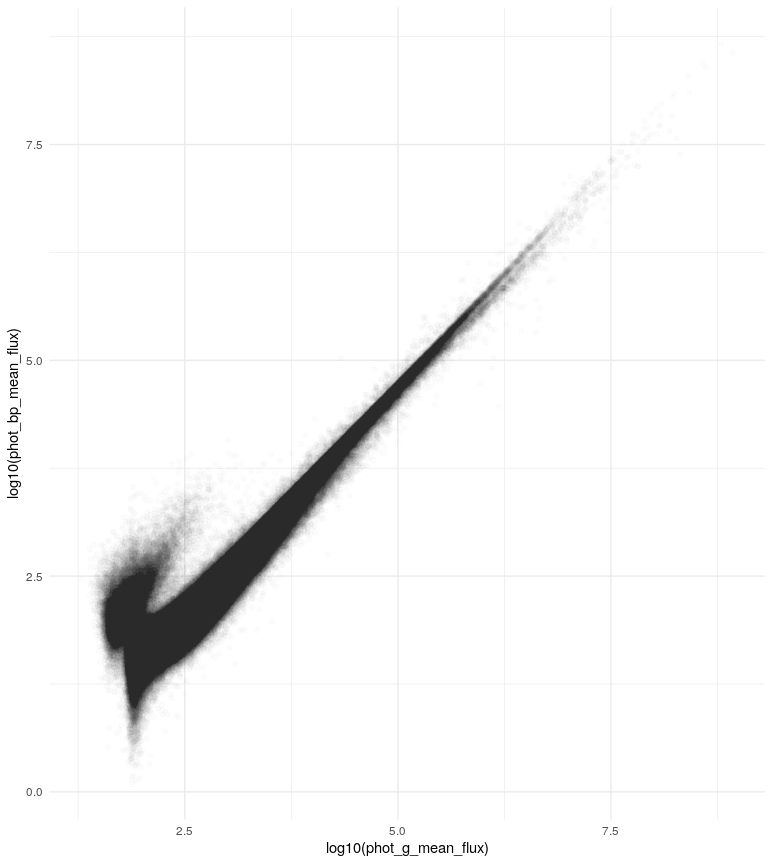
And here I’m plotting only two parameters of the 500K observations stored in just one file, so maybe the alien lasers are waiting for you on the database and remember: It is never aliens, until it is.
As always, the R scripts are available here.