Introduction.

A few months ago my wife told me that she wanted to try one of those fancy genetic tests that look for your ancestors, so you can know where they were from and even find distant cousins around the world. Despite I advised her against it because of privacy reasons. She insisted and I bought her a kit from MyHeritage (Don’t worry! what I am describing here this post applies to 23andme, ancestry, etc).
After receiving the results she immediately felt disappointed: just a few percentages relating her genes (or whatever they measure) with some populations around the globe. That was all!!!.
I was really curious about how those percentages were calculated and what they really meant. So I started analyzing the raw data that MyHeritage provides, a .csv file with the sequence of more than 600000 single nucleotide polymorphisms (SNPs). 600K SNPs to provide only a few percentages?? Are we crazy?! There is obviously much more than you can extract from that huge amount of information about yourself and in this post, I will give you some examples and guidelines for you to squeeze the maximum out of it. Indeed, while I was writing this post I received an advertisement from MyHeritage: Apparently now they also offer a new service called MyHeritage DNA Health+Ancestry kit. This is basically how it works, they perform the same genetic test and if you pay three times more, they analyze the data (the very same data) differently. Welcome to the new era of genomics, where it is cheaper to produce the data than to analyze it.

Genetic background.

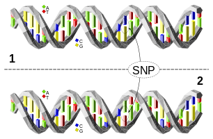
Let’s start from the beginning: What the hell is an SNP? and why you should care about them. We could say that genomes are the blueprint of life and the genes are the instructions to build every single living organism (it is not exactly like that, but it is a good proxy), that means that different organisms must have different blueprints, right? So the question is how different these blueprints are? You have probably heard many times things like “Humans share 85% of their DNA sequence with mice”. So if our blueprints and mice’s are 85% similar, how different are the DNA sequences between two humans? If we look at human beings the differences between us are very subtle compared with the human vs. mice ones (…of course). An answer for that is that most of the genes are the same among all human populations (and even Neanderthal), and the ones that are different, differ only in a tiny proportion. Here is where SNPs come in, one SNP is the minimum possible difference between two genes between two individuals and the sum of all the SNPs in our genomes is what makes us unique for bad or for good. Unfortunately, the role of the vast majority of human SNPs is unknown, however everyday science describes more and more SNPs, relating them to diseases or phenotypic traits so probably in a few years we will have a description for all the effects caused by every single SNP in the genome.

If you want a more technical definition, we could say that one SNP is a position in one nucleotide out of the 6.4·10^9 nucleotides that we have in our genomes, and for that particular nucleotide, there is one “reference” value (A, T, G or C) and one or more variant values which can be linked (or not) with certain phenotypes. To make things even more complex we need to consider that we humans are diploids, which means that we carry two copies of every SNP in the genome: one from your father and one from your mother so it is possible to have three combinations for each SNP: Reference-Reference, Reference-Variant, or Variant-Reference (A priori it is impossible to distinguish both of them in the results provided by MyHeritage) and Variant-Variant.

And each combination can have different traits, increasing the complexity of the story even more.

How do these genetic tests work, then?.

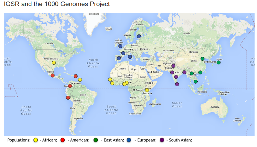
Now we know what SNPs are, but how can they help us to find our ancestors? To answer this question we need to talk about another characteristic of the DNA: its stability. The DNA is very very stable so it is very rare for mutations to happen and SNPs are just mutations in the genome that happened several thousands of years ago. Since human populations in the world were small and dispersed at that time it is possible to associate certain variants with certain ancient populations which can be divided in five big branches: African, European, American, South-Asian and East-Asian and for each SNPs, the percentage of individuals in each population carrying the variant form of the SNP varies. For instance, the reference nucleotide for the SNP rs10000008 located in the chromosome 4 position 172776204 is a C and the variant is a T, the frequency of the variant among the African population is 28.52% while the frequency among the European population is only 1.59%, that means that if you have a T it is more likely that you are African than European.

Note: If you are also interested in the methodological details of the test, I recommend you to read this paper: Microarray Based Genotyping: A Review

Statistical framework.

Now you have an idea about how the SNPs can help us to track our origins down; however, we still don’t know how the percentages provided by MyHeritage were obtained and what they really mean. Are they the probabilities of her belonging to each one of those populations? Are they the percentage of DNA associated with certain ethnicities? Are they something else? I don’t know and I am sure they are not going to disclose it. So we will need to perform our own analysis and compare our results with the report, but before doing it, we need to establish the statistical framework of the analyses.

There are several statistical approaches to analyze SNPs and in this post, I am going to compare frequentist and Bayesian strategies and to propose alternative ML-based analysis to solve the problems associated with them.
To do so we are going to use again the SNP rs10000008 as an example. Here is the list of all frequencies associated with the variant form (T) of that SNP:

AFR: 28.52%
EUR: 1.59%
SAS: 3.99%
EAS: 1.49%
AMR: 2.16%

So let’s say the result for a particular person is the presence of two copies of the variant form of that SNP (TT)… It is obvious that it is more likely for that person to be African, but how likely? Let’s see what the frequentist and Bayesian analyses say.

First of all, the frequencies provided by the 1000genomes consortium only account for the overall probability of having a variant (T), so we need to transform those probabilities into the probabilities of having each one of the three possible genotypes (CC, TC, and TT) and to do that we use these formulas:

${P(rs10000008=TT \cap ETH=AFR) = (rs10000008.AFR.Freq)^2 }$
${P(rs10000008=CC \cap ETH=AFR) = (1 - rs10000008.AFR.Freq)^2 }$
${P(rs10000008=TC \cap ETH=AFR) =2 \; rs10000008.AFR.Freq \; (1-rs10000008.AFR.Freq)}$

By applying the formulas we obtain these probabilities for TT:

AFR: 8.1%
EUR: 0.025%
SAS: 0.159%
EAS: 0.022%
AMR: 0.047%

So if we relativize the probabilities to add 100% (because we are 100% sure -in theory-) that the genotype is TT, we have the following percentages:

AFR: 96.97%
EUR: 0.30%
SAS: 1.9%
EAS: 0.26%
AMR: 0.56%

So the frequentist analysis tells us that if someone has a TT in the SNP rs10000008 his or her chances of being African are around 97%

Note: To achieve better accuracy we have to account for the sizes of the populations by multiplying those percentages by the ratio of the total population from that ethnicity.

Now, let’s see what the Bayesian analysis tells us. Bayesian analyses rely on the Bayes’ theorem:

\(P(A|B) = {P(B|A)· P(A) \over P(B)}\)

Applying that formula to our situation we have that:

P(A|B) is the conditional probability of A occurring given the fact B i.e: The probability of being African if you have the SNP rs10000008 equal to TT.

P(B|A) is the conditional probability of B occurring given the fact A i.e. The probability of rs10000008 is equal to TT among the African population

p(B) is the probability of B occurring i.e The overall probability of having a certain variant (rs10000008 equal to TT)

p(A) is the probability of A occurring i.e. The probability of being African

Before plugging the data that we already know, we have to define the distribution of populations around the globe, because we will use them as priors for our analysis:

AFR: 17%
EUR: 10%
SAS: 31%
MAR: 15%
EAS: 27%

What using P(A) = 0.17 actually means is that we don’t have any preconceptions about the result and since the 17% percent of the world population is African we assume that the probability of being African is 17% before obtaining the result. The power of Bayesian analyses is that we can modify our priors. Now imagine that we are taking the sample in the middle of Kinshasa, our prior for being African would be way higher. We could say that the Bayesian analysis computes how our beliefs (being African) should change after obtaining certain evidence (having a certain variant).

We plug in these values

P(B|A) = 8.1%
P(B) = 1.44% (The ponderated percentage for the variant)
P(A) = 17%

The calculation gives us 95.63%, which is pretty close to the result obtained using by a frequentist approach.

Well… We have used only one SNP to calculate the probability of belonging to a particular ethnic group. What are the rest of the SNPs used for then??! Well, we could make things more interesting by trying to combine all possible SNPs to give a more accurate probability; unfortunately, here is when both strategies fail…

The frequentist failure: To calculate the combined probability one could think that the multiplication of frequencies for all SNPs would do the trick, but it does not: The value gets smaller and smaller as it is multiplied by numbers lower than zero. That is because the real frequency of the combination of both is unknown and impossible to calculate it with the data that we have.

The Bayesian failure: To calculate the combined probability using Bayes’ theorem we need to expand the formula like this:

\[P(A|B \cap C) = {P(B \cap C|A)· P(A) \over P(B \cap C)}\]

However, there are a couple of problems: we don’t know the first element of the numerator and the denominator, so we need to pre-calculate them.

When two events are not ligated (I will come to point this out later) we can assume that:

\[P {P(B \cap C|A) = P(B|A)·P(C|A)}\]

And both terms are known.

Calculating the denominator is a bit more complicated, however, we know that:

\[P(A|B \cap C) = {P(B \cap C|A)· P(A) \over P(B \cap C)}\]

and

\[P(\sim A|B \cap C) = {P(B \cap C| \sim A)· P(\sim A) \over P(B \cap C)}\]

Which is the probability of not occurring A when B and C are occurring. As both probabilities are complementaries we can say that:

\[{P(A|B \cap C) + P(\sim A|B \cap C) = 1}\]

So we end up with the final equation:

\(P(A|B \cap C) = {P(B|A)·P(C|A)·P(A) \over P(B|A)·P(C|A)·P(A) + P(B| \sim A)·P(C| \sim A)·P(\sim A) }\)

For which we have all the information.

In this case, again we face a similar problem as in the frequentist approach, the numerator gets smaller and smaller with each SNP added, however, in theory, it shouldn’t be a problem because the denominator decreases in a similar range. However, in terms of computability, it becomes impracticable after a few hundred SNPs because even a machine can’t compute such small numbers.

Anyway, using hundreds of SNPs has to be better than using just one in order to obtain an accurate probability, right? Let’s compute it using R…

Analysis of populations using Bayes’ theorem in R

First, we need to perform some operations outside R since we need to get all the data that we need from the internet.

The web server that we are going to use is www.snp.nexus.org, where you can just send a list of SNPs and obtain several files containing information regarding them back; unfortunately, they only allow up to 100K SNPs per query, so we have to split our more than 600K SNPs into 7 files using R.

First, we load the raw data provided by MyHeritage and based on the number of SNPs we generate the files containing up to 100K SNPs in each.

#Data loading skipping the first 12 rows because they are comments in the file
df <- read.csv("/home/nacho/Raw_dna_data.csv", sep = ",", skip = 12)

#Generation of files for www.snp-nexus.org containing 100K SNPS
n.files <- round(nrow(df)/100000) + 1

for (i in 1:n.files){
  start<-((i-1)*100000)+1
  end<- min(i* 100000,nrow(df))
  dummy<-as.data.frame(rep("dbsnp", end-start+1))
  dummy$rsid<-df[start:end,1]

  write.table(dummy, file = paste("/home/nacho/SNPS_DB",i,".txt",sep = ""),
              col.names=FALSE,
              quote = FALSE,
              row.names = FALSE,
              sep = "\t")
}

Then, we upload them one by one into the server. The query takes around 14 hours to be processed, so it is a good idea to provide an email in the online form so you can receive an mail when the files are ready to download.

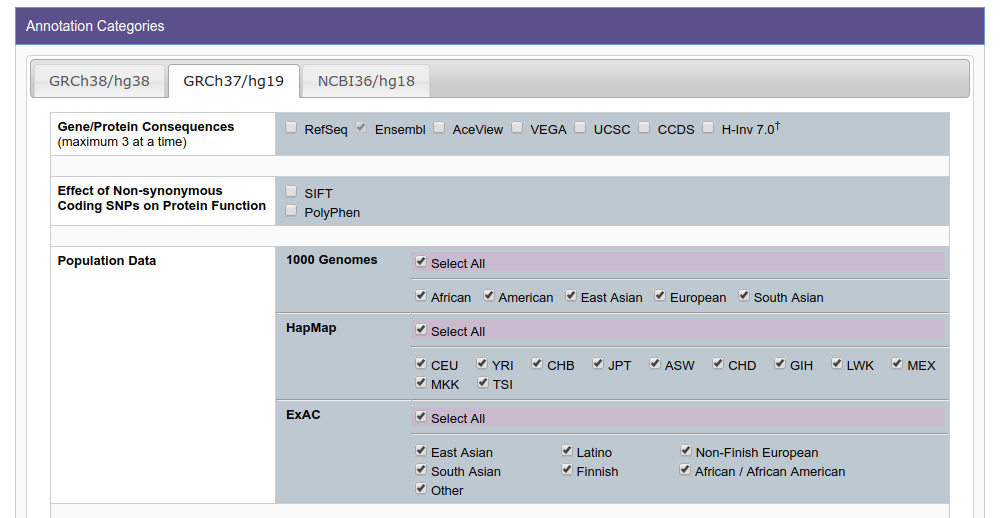
In the online form, you will find that there are many fields that you can request under the tab GRCh37/hg19. I suggest you to include at least these:

Population Data: ALL
Phenotype & Disease Association: ALL
Non-coding Scoring: ALL

With the unzipped files in your computer, it is time to prepare them, first, we need to rename them accordingly with the rename command from the terminal to have the names of the files with the same structure. This is a bit tedious but once you have them ready, it is very easy to merge them together into a big file that we can load in R. This is how the folder in my computer looks like:

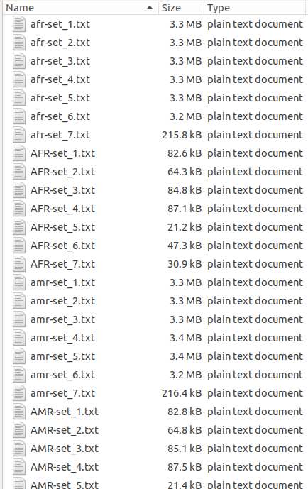
Once you have the files ready you can create a script in bash to merge all the files with the same structure together:

for file in  ???-*. C
  cat "$file" . C
  cat >>"${file%_*}.txt" . C
  cat
done

Note: There are many many ways of doing this process, here I’m just quickly describing the strategy that I used.

Now we can start importing the files into R:

#Populations loading 
path <- "/home/nacho/MyHerr/data/populations/"
files<-list.files(path)
setwd(path)

pop<-list()

pb <- txtProgressBar(min = 1, max = length(files), initial = 1) 
for (i in 1:length(files)) {
  setTxtProgressBar(pb,i)
  pop[[i]]<-read.csv(paste(path,files[i],sep = ""), sep = "\t")
}

#Subset populations 
files <- gsub("-.*","",files)

#1000genomes
code1000genomes<-c("afr", "eur", "sas", "amr", "eas")
pop1000genomes<-pop[which(files %in% code1000genomes)]
pop<-pop[-which(files %in% code1000genomes)]

#EAC
codeEAC<-c("AFR", "AMR", "OTH", "EAS", "FIN", "NFE", "SAS")
popEAC<-pop[which(files %in% codeEAC)]
pop<-pop[-which(files %in% codeEAC)]

Note that in order to distinguish the different datasets I have created two variables called code1000genomes and codeEAC, so all the files containing the ethnicity codes for each data set are loaded together into the same data frame. If you have changed the names of your files you will have to adjust code1000genomes and codeEAC accordingly. The last dataset (HapMap) is loaded just by removing the 1000genomes and EAC datasets from the list named pop

First, let’s assign the priors for each population and how they are distributed worldwide.

##### 1000genomes analysis 
#Merge data with sample 
priors1000genomes<- c(0.17, #afr
                      0.15, #amr
                      0.27, #eas
                      0.1,  #eur
                      0.31  #sas
                      )
                      

Now we can clean the data by removing duplicate elements and the SNPs in our results that were not available at www.snp.nexus.org](www.snp-nexus.org):

#Check that all of them are equal
rsid<-pop1000genomes[[1]]$SNP
for (i in 2:length(code1000genomes)) {
  rsid<-Reduce(intersect, list(pop1000genomes[[i]]$SNP, rsid ))  
}
rsid<- Reduce(intersect, list(df$RSID, rsid ))

df1000g<-subset(df, df$RSID %in% rsid )
df1000g<- df1000g[,c(1,4)]

Then, we replace the frequencies equal to 0 and 1 by 0.00005 and 0.99995 respectively. We do it because the frequencies in 1000genomes dataset are based on “few” samples, so it is very likely that those absolute values are not real and that there are some individuals carrying those variants in the whole population; indeed, 0.00005 is a very conservative estimation. If we assume that the 2504 samples of the 1000genomes project are evenly distributed, that gives us around 500 individuals per ethnicity. If the probability of a variant among the European population (the less represented worldwide speaking) is 0.00005 that means there would be 37070 European individuals carrying the variant and if we sample the population 500 times the probability of not getting any individual with that particular variant, and therefore assume that the frequency is 0, is higher than 98%. We also need to do that because Bayes doesn’t like zeroes, if we set a prior equal to zero in our computations the overall probability will be equal to zero.

  for (i in 1:length(code1000genomes)) {
    pop1000genomes[[i]]<-
    subset(pop1000genomes[[i]], pop1000genomes[[i]]$SNP %in% rsid)
    
   #changes zeros and ones
    
   pop1000genomes[[i]]$Frequency<-
   as.numeric(as.character(pop1000genomes[[i]]$Frequency))
   
   pop1000genomes[[i]]$Frequency[pop1000genomes[[i]]$Frequency==0]<-0.00005
   pop1000genomes[[i]]$Frequency[pop1000genomes[[i]]$Frequency==1]<-0.99995
   pop1000genomes[[i]]<-pop1000genomes[[i]][order(pop1000genomes[[i]]$SNP),]  
    }

We finish cleaning the data by creating new variables to account for the combined frequencies of the events in the rest of the populations (labeled as Rest in the code).

for (i in 1:length(code1000genomes)) {
  pop1000genomes[[i]][,c(2,3,7)]<-NULL
  
  colnames(pop1000genomes[[i]])<-paste(colnames(pop1000genomes[[i]]),
  code1000genomes[i],
  sep = "-")
  
  colnames(pop1000genomes[[i]])<- gsub("SNP-.*",
  "RSID", colnames(pop1000genomes[[i]]))
  
  #merging #Population size 5000
  if (i==1) df1000g <- merge( pop1000genomes[[i]],df1000g, by="RSID")
  if (i>1) df1000g <- cbind(df1000g,pop1000genomes[[i]] )

  list<- c(1:length(code1000genomes))
  list <- list[-i]
  
  Rest <- 0
  RestAlt1N<-0
  RestRef<-0
  
  for (h in 1:length(list)) {
  
#Modify rests
    Rest <- ((as.numeric(as.character(pop1000genomes[[list[h]]]$Frequency))^2) * priors1000genomes[[list[h]]]) + Rest
    
    RestAlt1N <- ((2*as.numeric(as.character(pop1000genomes[[list[h]]]$Frequency))-
                   2*as.numeric(as.character(pop1000genomes[[list[h]]]$Frequency))^2) * 
                   priors1000genomes[[list[h]]]) + RestAlt1N
    
    RestRef <- (1-2*as.numeric(as.character(pop1000genomes[[list[h]]]$Frequency))+
                  as.numeric(as.character(pop1000genomes[[list[h]]]$Frequency))^2) *
                  priors1000genomes[[list[h]]] + RestRef
  }
  
  df1000g$last<-Rest
  colnames(df1000g)[ncol(df1000g)] <- paste("Rest.2N.Alt",code1000genomes[i], sep = "-")
  df1000g$last<-RestAlt1N
  colnames(df1000g)[ncol(df1000g)] <- paste("Rest.1N.Alt",code1000genomes[i], sep = "-")
  df1000g$last<-RestRef
  colnames(df1000g)[ncol(df1000g)] <- paste("Rest.2N.Ref",code1000genomes[i], sep = "-")

  }

df1000g <- df1000g[complete.cases(df1000g),]

A bit more of data cleaning to remove those variant containing insertions/deletions (indels) and those that were not detected in the array (- -):

#remove non-detected SNPs
df1000g <- subset(df1000g,df1000g$RESULT!="--")
#remove indels
df1000g<-df1000g[which(nchar(as.character(df1000g$`Ref_Allele-afr`))==1),]
df1000g<-df1000g[which(nchar(as.character(df1000g$`Alt_Allele-afr`))==1),]
df1000g<-df1000g[which(nchar(as.character(df1000g$`Alt_Allele-eur`))==1),]
df1000g<-df1000g[which(nchar(as.character(df1000g$`Alt_Allele-sas`))==1),]
df1000g<-df1000g[which(nchar(as.character(df1000g$`Alt_Allele-amr`))==1),]
df1000g<-df1000g[which(nchar(as.character(df1000g$`Alt_Allele-eas`))==1),]

We also account for the diploids:

df1000g$Ref.2N <- paste(df1000g$`Ref_Allele-afr`, df1000g$`Ref_Allele-afr`, sep = "")

And calculate some probabilities (For the sake of simplicity I will only show the calculations for the African population, but you can find the complete script here)

#AFR
df1000g$Alt.1NA.afr <- paste(df1000g$`Ref_Allele-afr`, df1000g$`Alt_Allele-afr`, sep = "")
df1000g$Alt.1NB.afr <- paste( df1000g$`Alt_Allele-afr`, df1000g$`Ref_Allele-afr`, sep = "")
df1000g$Alt.2N.afr<-  paste(df1000g$`Alt_Allele-afr`, df1000g$`Alt_Allele-afr`, sep = "")
df1000g$Ref.2N.afr.Frq <- (1+ df1000g$`Frequency-afr`^ 2 - 2*df1000g$`Frequency-afr`)
df1000g$Alt.2N.afr.Frq <- df1000g$`Frequency-afr`^ 2

Then, we subset the dataset to separate the SNPs into heterozygous, homozygous reference and homozygous variants.

#AFR subsetting and calculation
df.afr.Ref.2N<- subset(df1000g[,c(1,4,5:8,37:42)], df1000g$RESULT==df1000g$Ref.2N)
df.afr.Alt.1N<- subset(df1000g[,c(1,4,5:8,37:42)], df1000g$RESULT==df1000g$Alt.1NA.afr |
df1000g$RESULT==df1000g$Alt.1NB.afr)  
df.afr.Alt.2N <- subset(df1000g[,c(1,4,5:8,37:42)], df1000g$RESULT==df1000g$Alt.2N.afr)

and we specify the priors again and the number of SNPs to be tested. Note: I have included the priors here again for testing purposes, alternatively, it would be very easy to recall the previous function and remap the values of the vector priors1000genomes into the new variables.

#Probability calculator
afr.priors <- 0.1
eur.priors <- 0.1
sas.priors<-0.3
amr.priors<-0.2
eas.priors<-0.3

N.elements<-150
#Probability calculator

Next, we create a matrix to compute the probabilities and select the SNPs randomly.

stats<- as.data.frame(array(data = NA, dim = c(N.elements,6)))
colnames(stats)<-c("N",code1000genomes)
rnd<-round(runif(1, min = N.elements, max = 50000))
  

Finally, we sequentially fill the matrix with the probabilities and the number of the SNPs analyzed.

for(n in 1:N.elements){
  stats$N[n]<-n*3

  #EUR
  num.eur<-eur.priors*
  prod(df.eur.Ref.2N$Ref.2N.eur.Frq[1:n+rnd])*
  prod(2*df.eur.Alt.1N$`Frequency-eur`[1:n+rnd] - 2*df.eur.Alt.1N$`Frequency-eur`[1:n+rnd]^2)*
  prod(df.eur.Alt.2N$Alt.2N.eur.Frq[1:n+rnd])

den.eur<-num.eur+
  ((1-eur.priors)*
     prod(df.eur.Ref.2N$`Rest.2N.Ref-eur`[1:n+rnd])*
     prod(df.eur.Alt.1N$`Rest.1N.Alt-eur`[1:n+rnd])*
     prod(df.eur.Alt.2N$`Rest.2N.Alt-eur`[1:n+rnd]))

prob.eur<- num.eur/den.eur

..........
..........

stats$afr[n]<-prob.afr
stats$eur[n]<-prob.eur
stats$sas[n]<-prob.sas
stats$eas[n]<-prob.eas
stats$amr[n]<-prob.amr

And we plot the results:

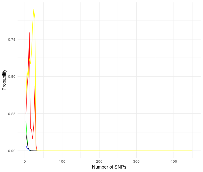
Wooow! Unexpected results, all probabilities collapse to zero after a few SNPs. As the 150 SNP to analyze are random I run it again.

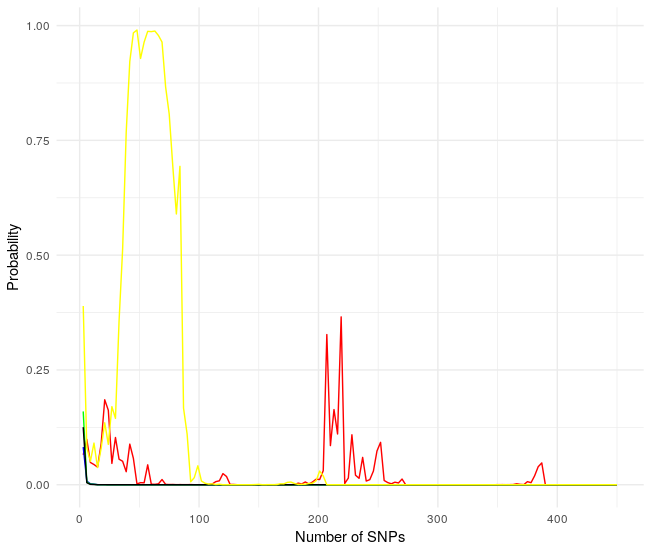
Same results! Probabilities collapse after a few SNPs but with a different profile. This is not the way to go because of the unpredictability.

Machine-learning framework.

Since pure statistical approaches seem to be unable to solve the usage of all SNPs to provide a result regarding the ethnicity of a sample I decided to implement an ML-based unsupervised clustering approach which takes into account the values of all SNP.

The idea is very simple. We know the probabilities associated with each variant for every ethnicity, so it should be possible to simulate the genotype of individuals for all SNPs. Then using unsupervised clustering we can find out where our sample clusters are.

To do that we first need to simulate the results of N individuals from every population:

library("cluster")
library("factoextra")
library("magrittr")

SampleSize<-20

Then we create a list with the number of SNPs that we want to use and a matrix containing the different individuals in rows, being the first one our sample. The genotype is encoded as 0: Homozygous reference, 1: Heterozygous and 2: Homozygous variant

RelevantSNP<-sample(as.character(df1000g$RSID),size = 4000, replace = FALSE)

population<-as.data.frame(matrix(data = NA, nrow = (SampleSize*5)+1, ncol = length(RelevantSNP) ))

dfpop<-subset(df1000g, df1000g$RSID %in% RelevantSNP)

dfpop$ploidy<-1
dfpop$ploidy[which(dfpop$RESULT==dfpop$Ref.2N)]<-0
dfpop$ploidy[which(dfpop$RESULT==dfpop$Alt.2N.afr)]<-2
population[1,]<-dfpop$ploidy
rownames(population)[1]<-"Sample"

Then iteratively we simulate the genotypes for each population like this:

pb <- txtProgressBar(min = 1, max = SampleSize*nrow(dfpop), initial = 1) 
count<-0

 #AFR generation
for (i in 2:(SampleSize+1)) {
  dfpop$dummy<-0
  for (h in 1:nrow(dfpop)) {
    count<-count+1
    setTxtProgressBar(pb,count)  
    rnd<-runif(1,min = 0, max = 1)
    if(rnd<dfpop$`Frequency-afr`[h]^2) dfpop$dummy[h]<-2
    if(rnd>(dfpop$`Frequency-afr`[h]^2) &
    rnd<(2*dfpop$`Frequency-afr`[h]-2*dfpop$`Frequency-afr`[h]^2)) dfpop$dummy[h]<-1     
  }
  population[i,]<-dfpop$dummy
  rownames(population)[i]<-paste("AFR",i,sep = "")

}

Once we have it, we can cluster the whole matrix row-wise using k-means:

k.clust<- kmeans(population, 5)
k.result<-k.clust$cluster
k.result<-as.data.frame(k.result)

And we can explore the group associated with the sample:

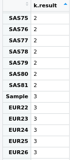
As you can see the sample clusters together with European simulated samples, something that in this case is totally expected.

If you want something more visual you can use other clustering methods that are better for hierarchical visualizations:

df.clust<-  dist(population,method = "binary")
df.clust<-hclust(df.clust,method = "ward.D2")  
fviz_dend(df.clust, k = 5,
          cex = 0.5, # label size         
          color_labels_by_k = TRUE, 
          rect = TRUE)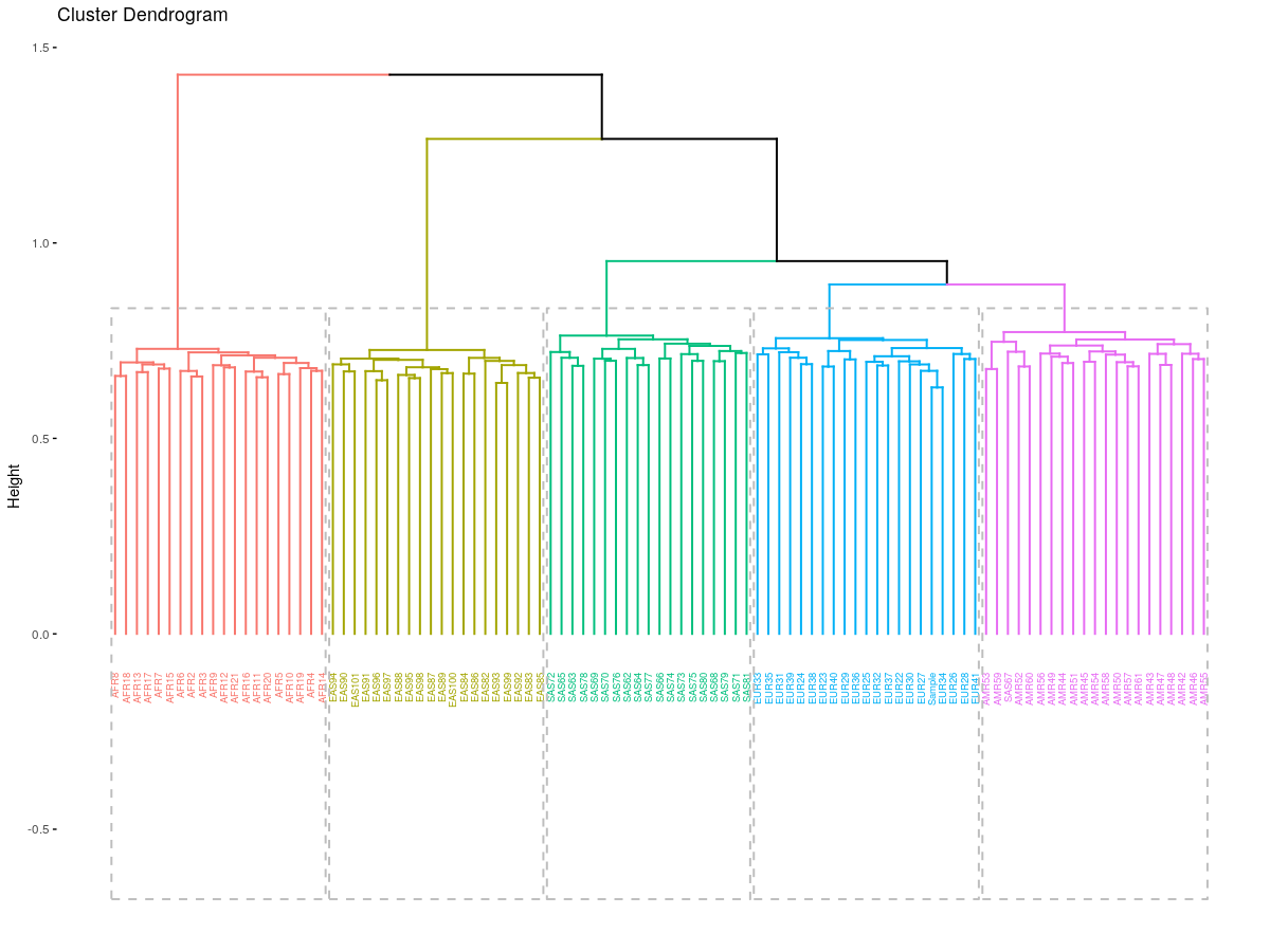

Here we have a better view of what is going on and how different groups correlate to each other, for instance, we can appreciate that the African population is more isolated (probably because it is the oldest).

As you can see, machine-learning strategies such as k-means perform much better than classical statistical approaches for genetic analyses. Of course, more SNPs would require longer computational times as well as a larger amount of simulations but nothing that a semi-decent computer can’t do in a few minutes, giving you more accurate results.

Although I don’t have a formal mathematical explanation for the difference in the performance I suspect that it might be related to the dependency of the variables. The Bayesian analyses as I intentionally mentioned, assume that the values are independent. However human SNPs are usually linked to each others, that means that some SNPs are inherited together so there is no independence. These groups of SNPs are what geneticists call haplotypes. It seems that somehow ML approaches are more flexible if we don’t account for the haplotypes-

Ethnicity calculation by DNA fragments.

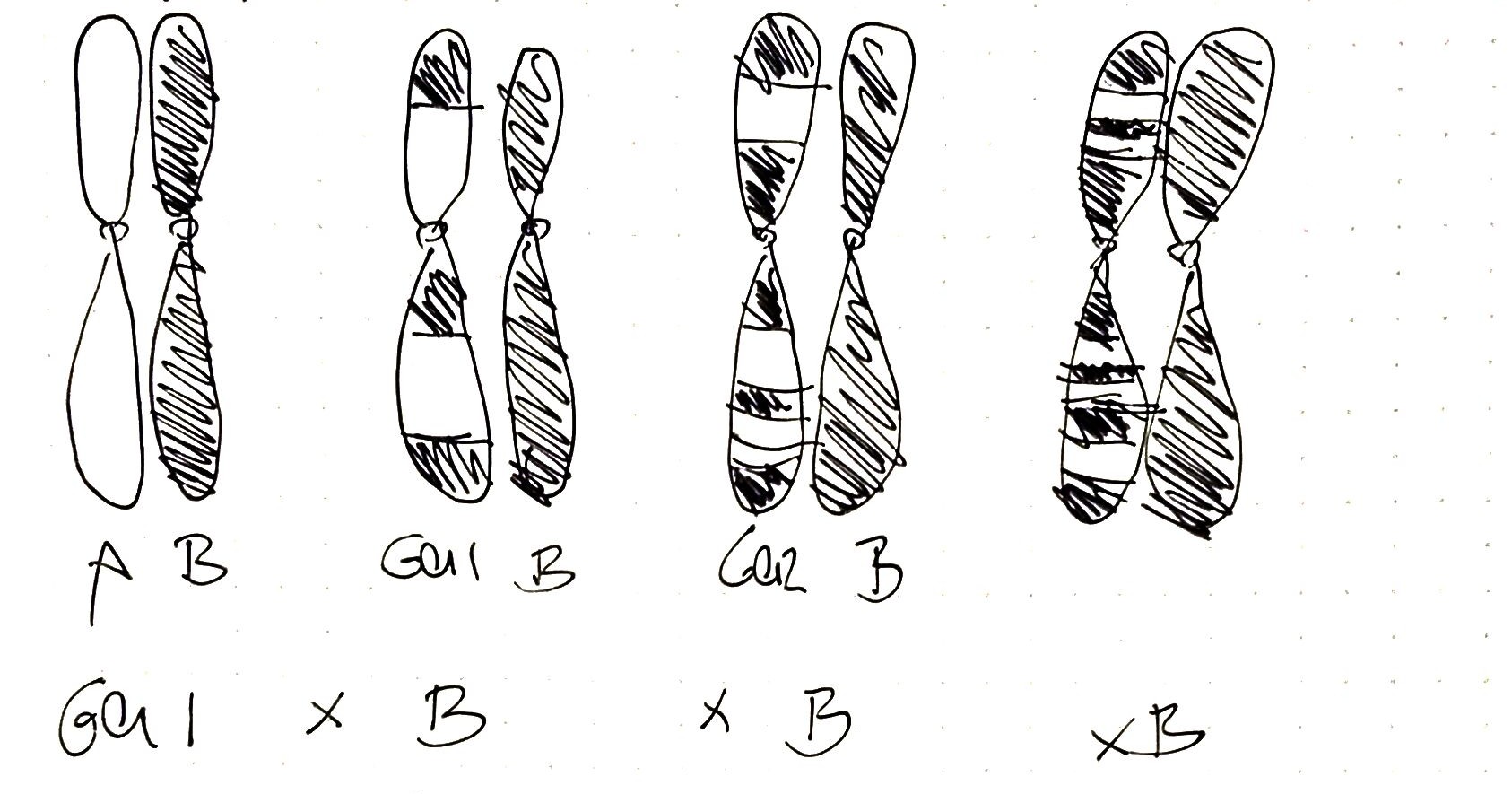
So far we have seen how to calculate the overall ethnicity of a person based on the results obtained from MyHeritage and in this section, we are going to split the whole genome into fragments and we are going to see if different fragments have different ethnicities. The rationale behind this analysis is that regions close in the genome tend to remain intact after several generations (they are linked). We could then say that the more fragmented the genome is (in terms of ethnicity) the more distant in time the sample is to that ancestor/s who carried that DNA fragment because of the meiotic recombination. Let’s say that we have two pure (ethnically speaking) ancestors A and B. If the offspring crosses again with a pure B the DNA content of the generation after will contain smaller fragments of A, if the second generation crosses with B again the A fragments will be even smaller… and so on so forth.

To do this analysis I am going to split the chromosomes into parts and the ethnicity of each part will be analyzed together with a score about the prediction. First I will use the unsupervised method explained before and then I will compare it with a frequentist approach.

First of all, we need to find the positions of the different SNPs in the genome, and to do that we need to cross our data with any of the 1000genomes datasets downloaded from www.snp.nexus.org.

#Load positions
positions<-read.csv("/home/nacho/MyHerr/data/populations/afr-set.txt",sep = "\t")
positions<-positions[,1:3]
colnames(positions)<-c("RSID","Chr","nt")
positions<-positions[!duplicated(positions$RSID),]
df1000g<-subset(df1000g,df1000g$RSID %in% unique(positions$RSID))
df1000g<-df1000g[!duplicated(df1000g$RSID),]
positions<-subset(positions, positions$RSID %in% unique(df1000g$RSID))

df1000g<-merge(df1000g,positions, by="RSID")

Then, to chop the chromosomes we need an additional file that you can find here. That file contains information regarding the chromosome size and the position of the centromere. Using that information we can divide the chromosome into pieces of a particular size, as stated in the variable genomic.size. For simplicity, we also rename chromosomes X and Y to 23 and 24.

genomic.size<-15000000
chr<-read.csv("/home/nacho/MyHerr/genome.txt.csv", sep = "\t",header = FALSE)
chr$chunks<-round(chr$V3/genomic.size)+1
chr$V1<-gsub("X","23",chr$V1)
chr$V1<-gsub("Y","24",chr$V1)

We create some empty columns in the data frame that will contain all the information once we fill in the array with a loop.

df1000g$nt<-as.numeric(as.character(df1000g$nt))
df1000g$Eth<-"ND"
df1000g$withinn<-NA
df1000g$cluster.score<-NA
df1000g$AFR.score<-NA
df1000g$EUR.score<-NA
df1000g$SAS.score<-NA
df1000g$AMR.score<-NA
df1000g$EAS.score<-NA

df1000g$Chr<-gsub("X","23", df1000g$Chr)
df1000g$Chr<-gsub("Y","24", df1000g$Chr)
df1000g$Chr<-as.numeric(df1000g$Chr)

and we define the number of individuals to be simulated for each set of SNPs

SampleSize<-25 #number of individuals for the clustering

To perform the clustering steps I am going to use parallel computing. Unless you do something about it, R-base performs all the task one by one using one processor (aka core) to run all the processes one after the other. However, nowadays most computers and even mobile phones have more than one core, so running the code in such a way is a waste of resources and time. To optimize the code we can perform what it is called parallel computing, that means that we split the whole computational task into smaller subtasks and we assign each one of them to a core to be processed.

This is what the computer does when you run this analysis without any parallelization:

and this is what the computer does when you parallelize the analysis:

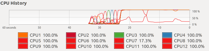
As you can imagine it is much more efficient to have 11 cores working in the same process than 1 core doing all the tasks, and indeed it divides the computing time by 10.

As a rule of thumb, when you are doing parallel computing you always divide the larger tasks to be performed, which usually means replacing the external loop (for/while/etc) by the parallelizing function foreach()%dopar%

However, before performing the analysis we need to prepare the set of cores (aka cluster) that we are going to use. We load the libraries, detect the total number of cores in the machine (N) and create the cluster with N-1 cores, otherwise, you couldn’t use the computer while the computation is running.

library(doParallel)
library(parallel)
library(foreach)
cores<-detectCores()-1
cluster.cores<-makeCluster(cores)
registerDoParallel(cluster.cores)

Then, we define the parallelization loop pointing to a variable which after the computation will be of the type list. In each element of the list, there will be the result of the computation performed by one core. This is done in this way because when the computer creates the cluster it also creates a copy of the variables to be used for each core in a way that the cores don’t know what is going on with the other cores, so after the computation we need to wrap it up and combine the results from all the cores.

In this particular case, the loop splits the task in chromosomes: each chromosome for a core. Then, each core chops the chromosome according to the desired sampling size and computes the clustering. We obtain the ethnicity by calculating the mode of the ethnicity of the simulations that cluster together with our sample of interest; in other words, if most of the simulations that cluster together with our sample are European we assign the European ethnicity to that DNA fragment. We compute the median with the function:getmode (source of the idea).

getmode <- function(v) {
  uniqv <- unique(v)
  uniqv[which.max(tabulate(match(v, uniqv)))]
}

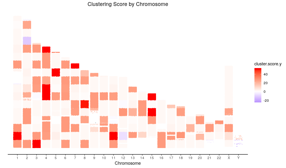
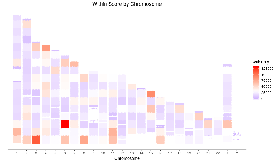
To assess the accuracy of the prediction, I have included a couple of scores in the script stated in the columns df1000g$withinn and df1000g$cluster.score. The first one accounts for the withinnes of the cluster containing the sample of interest, the lower the value the better, although there are circumstances in which larger values don’t mean worse predictions. The second score somehow accounts for the misclassification of the simulations in the cluster containing the sample, a perfect classification gives a value of zero (although some misclassifications have a score equal to zero) a deviation to a positive number means that the cluster is including incorrect simulations and a negative number means that the cluster is not accounting for all the simulations generated for a particular ethnicity. In a nutshell, it is optimal at zero and then a negative value is preferred because the higher the value the higher the probability of misclassification of the sample.

output<-foreach(i2=1:nrow(chr), .verbose = TRUE, .packages = "cluster") %dopar%{

  chr.tolook<-paste("chr",i2,sep = "")
  chunks<-chr$chunks[chr$V1==chr.tolook]  
  #print(paste("Analyzing Chr",i2,sep=""))
  #pb <- txtProgressBar(min = 1, max = chunks, initial = 1) 
  for (h2 in 1:chunks) {
    #setTxtProgressBar(pb,h2)   
    RelevantSNP<-
    as.character(df1000g$RSID[df1000g$nt >
    (h2-1)*genomic.size & df1000g$nt <
    h2*genomic.size & df1000g$Chr==i2])
    
    if(length(RelevantSNP)>1){
    dfpop<-subset(df1000g, df1000g$RSID %in% RelevantSNP)
    dfpop$ploidy<-1
    dfpop$ploidy[which(dfpop$RESULT==dfpop$Ref2N)]<-0
    dfpop$ploidy[which(dfpop$RESULT==dfpop$Alt2N)]<-2
    
    population<-as.data.frame(matrix(data = NA, nrow = (SampleSize*5)+1, ncol = length(RelevantSNP) ))
    
    population[1,]<-dfpop$ploidy
    rownames(population)[1]<-"Sample"
    
    EthScore<-rep(NA, length(code1000genomes))
  
    #AFR generation
    for (i in 2:(SampleSize+1)) {
      dfpop$dummy<-0
      for (h in 1:nrow(dfpop)) {
        rnd<-runif(1,min = 0, max = 1)
        if(rnd<dfpop$`Frequency-afr`[h]^2) dfpop$dummy[h]<-2
        if(rnd>(dfpop$`Frequency-afr`[h]^2) &
        rnd<(2*dfpop$`Frequency-afr`[h]-2*dfpop$`Frequency-afr`[h]^2)) dfpop$dummy[h]<-1     
      }
      population[i,]<-dfpop$dummy
      rownames(population)[i]<-paste("AFR",i,sep = "")
      
    }

    #EUR generation
    for (i in (SampleSize+2):(2*SampleSize+1)) {
      dfpop$dummy<-0
      for (h in 1:nrow(dfpop)) {
        rnd<-runif(1,min = 0, max = 1)
        if(rnd<dfpop$`Frequency-eur`[h]^2) dfpop$dummy[h]<-2
        if(rnd>(dfpop$`Frequency-eur`[h]^2) &
        rnd<(2*dfpop$`Frequency-eur`[h]-2*dfpop$`Frequency-eur`[h]^2)) dfpop$dummy[h]<-1     
      }
      population[i,]<-dfpop$dummy
      rownames(population)[i]<-paste("EUR",i,sep = "")
      
    }
    
    #AMR generation
    for (i in (2*SampleSize+2):(3*SampleSize+1)) {
      dfpop$dummy<-0
      for (h in 1:nrow(dfpop)) {
        rnd<-runif(1,min = 0, max = 1)
        if(rnd<dfpop$`Frequency-amr`[h]^2) dfpop$dummy[h]<-2
        if(rnd>(dfpop$`Frequency-amr`[h]^2) &
        rnd<(2*dfpop$`Frequency-amr`[h]-2*dfpop$`Frequency-amr`[h]^2)) dfpop$dummy[h]<-1     
      }
      population[i,]<-dfpop$dummy
      rownames(population)[i]<-paste("AMR",i,sep = "")
      
    }
    
    #SAS generation
    for (i in (3*SampleSize+2):(4*SampleSize+1)) {
      dfpop$dummy<-0
      for (h in 1:nrow(dfpop)) {
        rnd<-runif(1,min = 0, max = 1)
        if(rnd<dfpop$`Frequency-sas`[h]^2) dfpop$dummy[h]<-2
        if(rnd>(dfpop$`Frequency-sas`[h]^2) &
        rnd<(2*dfpop$`Frequency-sas`[h]-2*dfpop$`Frequency-sas`[h]^2)) dfpop$dummy[h]<-1     
      }
      population[i,]<-dfpop$dummy
      rownames(population)[i]<-paste("SAS",i,sep = "")
      
    }
    
    #EAS generation
    for (i in (4*SampleSize+2):(5*SampleSize+1)) {
      dfpop$dummy<-0
      for (h in 1:nrow(dfpop)) {
        rnd<-runif(1,min = 0, max = 1)
        if(rnd<dfpop$`Frequency-eas`[h]^2) dfpop$dummy[h]<-2
        if(rnd>(dfpop$`Frequency-eas`[h]^2) &
        rnd<(2*dfpop$`Frequency-eas`[h]-2*dfpop$`Frequency-eas`[h]^2)) dfpop$dummy[h]<-1     
      }
      population[i,]<-dfpop$dummy
      rownames(population)[i]<-paste("EAS",i,sep = "")
      
    }
    
    k.clust<- kmeans(population, 5)
    k.result<-k.clust$cluster
    k.result<-as.data.frame(k.result)
    
    cluster<-rownames(k.result)[k.result$k.result== k.result[1,1]]
    
    cluster<-cluster[-1]
    cluster<-gsub("\\d","",cluster)

    df1000g$Eth[df1000g$RSID %in% RelevantSNP]<-getmode(cluster)
    df1000g$withinn[df1000g$RSID %in% RelevantSNP] <- k.clust$withinss[as.numeric(k.clust$cluster[1])]
    df1000g$cluster.score[df1000g$RSID %in% RelevantSNP] <- k.clust$size[k.clust$cluster[1]]-SampleSize+1

    rm(cluster)
    
    }#If there are SNP in the region
    
  }#Chunks
  
  return(subset(df1000g[c("RSID","Eth","cluster.score","withinn")], df1000g$Chr==i2))
  
}#chr

stopCluster(cluster.cores)

Finally, we wrap the output out.

Note: this is not necessary if you stated in the cluster that you want all the results rbinded but I prefer to do it in this way to be able to inspect the list and troubleshoot any possible error (since you can’t inspect any modification in the variables after they are assigned to the cluster it is difficult to trace back errors occurring in the cluster)

out<-rbind(output[[1]],output[[2]])
for (i in 3:length(output)){
  out<-rbind(out,output[[i]])
  }

df1000g<-merge(df1000g,out, by="RSID")  

Now we are ready to plot the results.

ggplot(subset(df1000g))+
  geom_jitter(aes(x=as.numeric(as.character(Chr)), y=nt, colour=Eth.y),size=0.05)+
  #geom_rect(aes(xmin=0.5, xmax=1.5, ymin=0, ymax=10000000), color="black", alpha=0) +
  ggtitle("Ethniticity by Chromosome")+
  xlab("Chromosome")+
  ylab(" ")+
  scale_x_discrete(limits=c(1:24), labels=c(1:22,"X","Y"))+
  scale_y_continuous(breaks=NULL)+
  theme_classic()+
  theme(plot.title = element_text(hjust = 0.5))

For privacy reasons, I am not plotting the ethnicity by chromosome but instead, I am plotting the scores for each ethnicity:

Now I am going to perform an analogous analysis but using a frequentist approach instead. To do that, we first need to define a genetic score for each ethnicity in a way that the higher the genetic score is the higher the chances of an ethnicity prediction to be correct.

I have devised a genetic score in which we calculate the difference in the probability of having a certain SNP between a population and the rest of the population. If that mutation is more likely to happen in the selected population the value is positive and negative if it is less likely. The higher the value (positive or negative) the higher the importance of that SNP to calculate the score, then we only have to calculate the mean of the scores for every SNP in the region that we are investigating and repeat it for every population, the population with the higher positive score is the one assigned to that region.

I have encoded the genetic score into this function:

  GenScore <- function(ploidy, Freq, Rest.Freq){
    Score<-rep(NA,length(Freq))
    Dip.Var <- Freq^2
    Dip.Ref <- (1-Freq)^2
    Hap<- 2*Freq*(1-Freq)
    
    Rest.Dip.Var <- Rest.Freq^2
    Rest.Dip.Ref <- (1-Rest.Freq)^2
    Rest.Hap<- 2*Rest.Freq*(1-Rest.Freq)
    
    Score[which(ploidy==2)]<- Dip.Var[which(ploidy==2)] - Rest.Dip.Var[which(ploidy==2)]
    Score[which(ploidy==0)]<- Dip.Ref[which(ploidy==0)] - Rest.Dip.Ref[which(ploidy==0)]
    Score[which(ploidy==1)]<- Hap[which(ploidy==1)] - Rest.Hap[which(ploidy==1)]
    
    return(Score)
    
  }

So we only need to call it during each iteration.

  #AFR
    Freq <- dfpop$`Frequency-afr`
    Rest.Freq <- dfpop$Anti.AFR
    EthScore[1]<-mean(GenScore(ploidy, Freq, Rest.Freq),na.rm = TRUE)

After plotting the results (that I am not showing for privacy reasons) I have found that most of the predicted regions in the chromosomes are quite similar; however, the unsupervised clustering approach seems to be more precise.

Here is how the plot of the European score looks like:

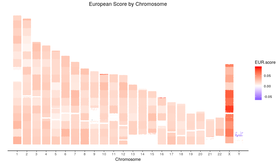
Interestingly, I have found that the scores in the X chromosome look higher than in the rest of the chromosomes, if we look at other ethnicities we can find that indeed the values are more extreme than in the rest of the genome. Now, considering that the genetic score measures differences in probabilities, that could indicate that such differences are higher at chromosome X. Does this make any sense? Is it an artifact? It is difficult to tell without any other samples to compare. A hypothesis is that since half of the samples (the males) only have one copy of the chromosome X there is an alteration in the frequencies that makes the differences higher.

Conclusions and future work.

In this post, we have seen how to analyze our own genetic data provided by MyHeritage, 23andMe, Ancestry, etc… We have seen that there is much more information hidden in the raw data and we have set a framework to study such information.

In the future, I will write about how to analyze predisposition to certain diseases based on the data provided. I will also include a more complete genetic study such as HapMap in which there are many more ethnicities than in the 1000genomes. If you are looking forward to squeezing your genetic data, stay tuned!