Introduction.

For millions of years, evolution has selected and improved the human ability to recognize faces. Yes! We, humans, are one of the few mammals able to recognize faces, and we are very good at it. During the courses of our lives, we remember around 5000 faces that we can later recall despite poor illumination conditions, major changes such as strong facial expressions, the presence of beards, glasses, hats, etc… The ability to recognize a face is one of those hard-encoded capabilities of our brains. Nobody taught you how to recognize a face, it is something that you just can do without knowing how.

Despite this apparent simplicity, to train a computer to recognize a face is an extremely complex task mainly because faces are indeed very similar. All faces follow the same patterns: there have two eyes, two ears, a nose and a mouth in the same areas. What makes faces recognizable are milimetrical diferences, so how can we train a machine to recognize those details? Easy, using convolutional neural networks (CNNs).

CNNs.

CNNs are special types of neural networks in which the data is processed by one or several convolutional layers before being fed into a classical neural network. A convolutional layer processes each value of the input differently, depending on the neighboring data. If we are talking of images, the processed value for each pixel of the image will depend on the surrounding pixels and the rules to process them are what we call filters.

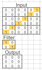
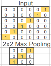
One of the main features of convolutional layers is that they are very good at finding patterns. Let’s see how they work with a simple, but very intuitive, example: Imagine a picture of 6x6 pixels and a bit-depth of 2. One of the few shapes that it is possible to draw in such a rudimentary system is a diagonal line and. Indeed, there are two possible diagonal lines ascending and descending ones. It is possible to devise a simple convolutional layer consisting of one single filter that finds descending diagonals in the picture ignoring the ascending ones:

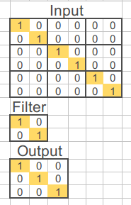
The output image is the result of multiplying the values of the input by the filter in the different areas of the image covered by the filter. If the CNN finds the pattern, the pattern is preserved; otherwise, it is filtered out:

Of course, CNNs are much more complex than this. The filter can slide through the matrix pixel by pixel, the values obtained after applying the filter can be added together, etc… however, the concept is exactly the same.

So the idea behind a face recognition algorithm is to send the images through several convolutional layers to find the patterns that are unique for each person and link them to the identity of the subject through a neural net that we can train. {: style=”text-align: justify”}

The Olivetti face database.

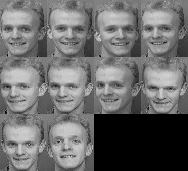
Since I just wanted to play around with these concepts testing different models, I needed a small database so I didn’t spend several hours training a model each time that I wanted to change a parameter. For that purpose the Olivetti database is perfect, it consists of 400 B/W images from 10 different subjects. The images are 92 x 114 with 256 tones of grey (8 bits). You can download the original dataset from the AT&T lab here or a version ready-to-use here (The version ready-to-use is exactly the same as the original one but for simplicity, it contains all the images in the same folder with the number of the subject already encoded in the name of the file).

This is basically how the 10 images for one of the subjects (#5 in this case) look like:

Loading of images into the R environment.

If you are using the ready-to-use file you will find that the images have this name structure SX-Y.pgm where X is the number of the subject and Y the number of the picture. So once you have all the images ready in the same folder you can load them into R using something like this:

library(imager)

Path<-"/home/nacho/ML/faces/"

files<-list.files(Path)
setwd(Path)

df.temp <- load.image(files[1])
df.temp <- as.matrix(df.temp)

df<-array(data = 0,
          dim = c(length(files),nrow(df.temp),ncol(df.temp),1))

for (i in 2:length(files)) {
  df.temp <- load.image(files[i])
  df.temp <- as.matrix(df.temp)
  df[i,,,1] <- df.temp
   }

First, the script uses the imager library and the path where the images are located as a variable. Next, in order to make the script working independently of the number of the images in the dataset, the first image in the folder is loaded, transformed into a matrix and accommodated into an array with 4 dimensions: Number of images, height, width and 1 (since the images are b/w, one channel is enough the describe the color depth). Finally, all the images are sequentially loaded into the array with a for() loop.

By inspecting the array it is possible to see that all the grey values have already been normalized so the maximum possible white value is 1. To visualize the images in R you can use the image() function like this:

image(df[1,,,],
        useRaster = TRUE,
        axes=FALSE,
        col = gray.colors(256, start = 0,
        end = 1,
        gamma = 2.2,
        alpha = NULL))

This code reconstructs the first image stored in the array (df[1,,,]) to produce this plot:

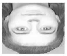
It seems that the data is loaded upside down in the array, but I don’t really care since this inversion is common to all the images in the array.

Next, I prepared the dependent variable to be matched with each image during the training step. To do that I extracted the number of the subject from the name of the file:

Y <- gsub(" .*","",files)
Y <- gsub("s","",Y)

The last step before constructing the model is to divide the dataset into training and testing. I decided to use 9 images of each subject for the training process and the remaining image for testing purposes. The number in the sequence of pictures for testing is the same for all subjects and it is randomly defined.

#Training and test datasets
TestSeq<-(c(1:40)*10)+round(runif(1, min = 1, max = 10))-10

x_test <- df[TestSeq,,,1]
y_test <- Y[TestSeq]  
x_train <- df[-TestSeq,,,1]
y_train <- Y[-TestSeq]

Building the model.

To construct the model I used Keras, which is a very flexible and powerful library for machine learning. Although most of the tutorials and examples over the internet about Keras are based on Python, it is possible to use the library in R and this is what I am going to explain in this post.

As usual, the first time you use Keras you have to install the library:

devtools::install_github("rstudio/keras")
library(keras)
install_keras()

These commands will install Keras and TensorFlow, which is the core of Keras. Once Keras has been installed it is possible to load it like the rest of the R libraries with library(keras)

With Keras it is possible to create recursive models in which some layers are reused or models with several inputs/output but the most simple and common type of models are the sequential models. In a sequential model, the data flows through the different layers to end up in the output layer where it is compared with the dependent variable during the training.

This face recognition model is a sequential model in which the data extracted from the images is transformed through the different layers to be compared in the last layer with the dependent variable to tune the weights of the model in order to minimize the loss function.

#Model 
model <-keras_model_sequential()

The use of the pipe operator %>% (Ctrl+Sift+M in RStudio) is extremely useful to add the different layers that conform the model:

model %>%
  #CNN part
  layer_conv_2d(filter=32,
  kernel_size=c(3,3),padding="same",input_shape=c(92,112,1) ) %>%  
  layer_activation("relu") %>%  
  layer_conv_2d(filter=32 ,kernel_size=c(3,3))  %>%  
  layer_activation("relu") %>%
  layer_max_pooling_2d(pool_size = c(2,2)) %>% 

In the CNN part, the data enters into a 2D convolutional layer with 32 filters of 3x3 size. In this layer the shape of the data is also defined by input_shape=c(width, height, channels). As activation function, I used the most common one in CNNs, which is ReLU. Then the data from the first CNN is processed by a second CNN to find patterns of a higher order. Finally, a max pooling layer is added for regularization. In this layer, it occurs downsampling of the data that also prevents overfitting. The pool size is 2x2, that means that the matrix is aggregated in a 2-by-2 manner and that the maximum value of the 4 pixels is selected:

Now, let’s look at the neural network section:

#Neural-net part 
  layer_flatten() %>% 
  layer_dense(1024) %>%
  layer_activation("relu") %>% 
  layer_dense(128) %>% 
  layer_activation("relu") %>% 
  layer_dropout(0.3) %>% 
  layer_dense(40) %>% 
  layer_activation("softmax")

First, the data coming from the CNN is flattened, meaning that the array is reshaped into a vector with only one dimension. Then, the data is sent through two fully-connected layers of 1024 and 128 neurons with ReLU again as the activation function. Next, a regularization layer is added to drop out 30% of the neurons. Finally, an output layer with the same number of units as elements to classify (40 in this case) is added, the activation function of this layer is softmax, that means that for each prediction the probability of belonging to each one of the 40 classes is calculated.

Once the model is created it is possible to visualize it using summary(model)

________________________________________________________________
Layer (type)                   Output Shape          Param #             
================================================================
conv2d_3 (Conv2D)             (None, 92, 112, 32)      320                 
_________________________________________________________________
activation_6 (Activation)     (None, 92, 112, 32)      0                   
_________________________________________________________________
conv2d_4 (Conv2D)             (None, 90, 110, 32)      9248                
_________________________________________________________________
activation_7 (Activation)     (None, 90, 110, 32)      0                   
_________________________________________________________________
max_pooling2d_2 (MaxPooling2D)(None, 45, 55, 32)       0                   
_________________________________________________________________
flatten_2 (Flatten)           (None, 79200)            0                   
_________________________________________________________________
dense_4 (Dense)               (None, 1024)             81101824            
_________________________________________________________________
activation_8 (Activation)     (None, 1024)             0                   
_________________________________________________________________
dense_5 (Dense)               (None, 128)              131200              
_________________________________________________________________
activation_9 (Activation)     (None, 128)              0                   
_________________________________________________________________
dropout_2 (Dropout)           (None, 128)              0                   
_________________________________________________________________
dense_6 (Dense)               (None, 40)               5160                
_________________________________________________________________
activation_10 (Activation)    (None, 40)               0                   
=================================================================
Total params: 81,247,752
Trainable params: 81,247,752
Non-trainable params: 0
_________________________________________________________________

The next step is to compile the model with the optimization parameters and the loss function:

opt<-optimizer_adam( lr= 0.0001 , decay = 1e-6 )
compile(model,optimizer = opt, loss = 'categorical_crossentropy' )

For the optimization, I am using the Adam optimizer which is one of the state-of-the-art algorithms for weight tuning commonly used in image classification. The loss function here will be the cross-entropy. Here you can read more about the Adam optimizer and here you can read an interesting post where the author explains very well the cross-entropy.

There is one last step before training the model which is to do one-hot-encoding of the dependent variable. One-hot-encoding is an alternative way of representing the dependent variable in opposition to the label-encoding, which is the traditional way of showing it:

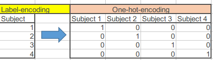
The to_categorical() function from Keras can do the job:

y_train <- to_categorical(y_train)
y_test <- to_categorical(y_test)

It is finally time to train the model:

history<-model %>% fit(x_train, y_train,
              batch_size=10,
              epoch=10,
              validation_data = list(x_test, y_test),
              callbacks = callback_tensorboard("logs/run_a"),
              view_metrics=TRUE,
              shuffle=TRUE)

The important parameters here are the batch size which is the number of samples that are processed before the model is updated and the number of epochs which is the number of times that the entire dataset goes through the model. I set both to 10 as an starting point.

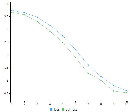
After 10 minutes of training in my slow computer (i5-4200U/4Gb) the model achieves an impressive 92.5% prediction accuracy, with only 3 faces misclassified. This is an awesome score, considering that the model had only 9 samples to train on and it only had run through the whole dataset 10 times. Moreover, by looking at the shape of the training curve it is possible to anticipate that more epochs would lead to better predictions.

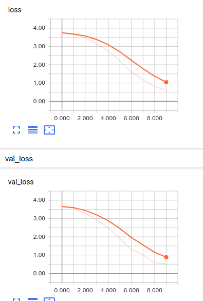
Another amazing feature of Keras/TensorFlow is the possibility of using TensorBoard, a kind of front-end for TensorFlow, which shows a lot of information presented in a beautiful way.

Conclusions.

In this post, we have seen a very basic example of image recognition and classification in R with Keras. Using this playground it is possible to implement advanced models to solve more complex image-classification tasks. I hope you enjoy it as much as I did.

As always you can download the code of this post Here

Bibliography and Sources of Inspiration.

Keras for R
How to implement Deep Learning in R using Keras and Tensorflow