Introduction

We humans learned how to use drugs many thousands of years ago. The shaman of the tribe already knew which roots and plants had healing effects on sick people. Of course, he didn’t know of anything about chemistry or why they worked, but it was the pre-scientific era, so who cared?!

Slowly, mankind became better at using drugs, but only as a consequence of a long trial and error process and it was not until the scientific revolution when we started an active and systematic search for new medicines which, together with the advances in chemistry and biology, lead us to a golden age of medicine in the middle of the 20th century when there was an explosion in the number of antibiotics, anticancer and antifungal treatments. It seemed that in a few years we would be able to cure anything. Unfortunately, that was not the case, fungi and bacteria are becoming resistant to treatments and anticancer therapies are still ineffective and unspecific. Moreover, the drug-discovery pipeline is still slow and inefficient and since the number of drugs-to-be-found is finite, it is becoming more and more difficult to find novel bioactive-chemicals, making the process extremely expensive.

We clearly need new approaches to speed up the process of drug discovery and in these series of posts, I will present some ideas about using ML and AI to reach that goal.

The rationale behind using ML to find drugs

When we train a ML model we are creating an “algorithm” that learns a function f(x)=y. In our case the function that we want to learn is simple: f(drug)=activity and the hypothesis to test is that “if we can learn (or approximate) the f(drug)=activity function we can instantly predict the activity of a drug without testing it in the lab”. So if this hypothesis is true it would save thousands of hours and tons of money in the drug-discovery process.

The first thing to do to approximate the function f(drug)=activity is to parameterize the two terms of the function.

The parameterization of the activity is easy because we can quantify it: it can be, for instance, the EC50, which is the concentration at which the drug achieves half of the maximum effect, it can be the pKi, which is a measurement of the strength of a drug-protein interaction or it can be the area under certain activity curve. It can be continuous ranging between two values or discrete with two or more classes (e.g. no-activity, moderate-activity, high-activity). It doesn’t really matter as long as it is measurable and meaningful to make inferences about unknown drugs.

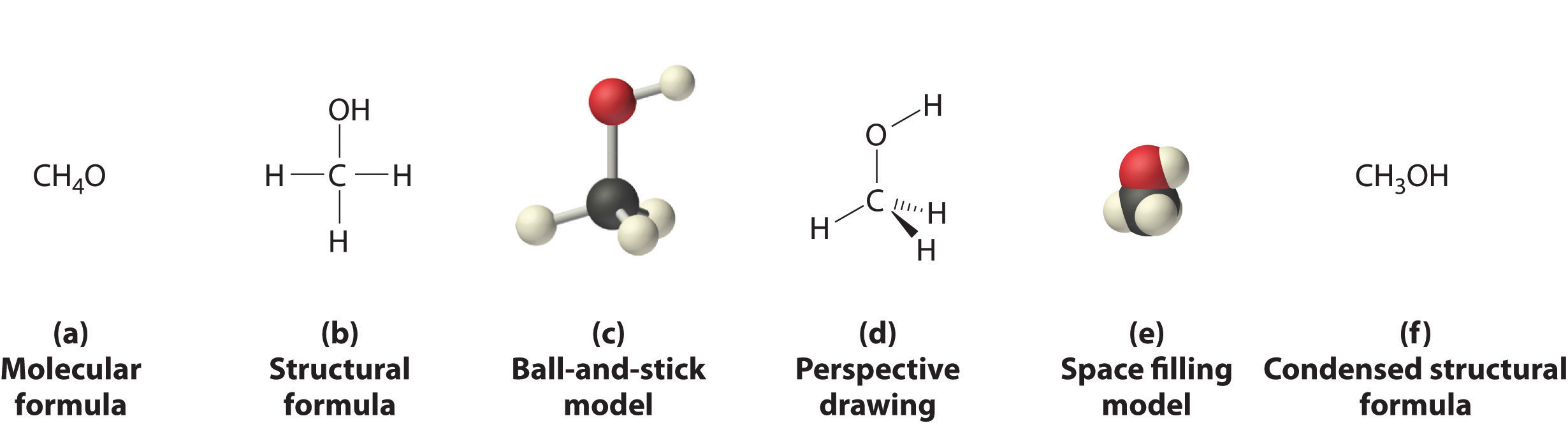
The parameterization of the drugs is much more complex and it first requires to find a suitable way to represent the compounds. Although there are many ways of representing a drug (e.g. Molecular and structural formulas, balls-and-sticks, space-filling) all of them have downsides due to loss of information (e.g. loss of 3D information) or wrong assumptions (e.g. all bonds having a similar length). Additionally, these representations are very difficult to parameterize.

Drug representation

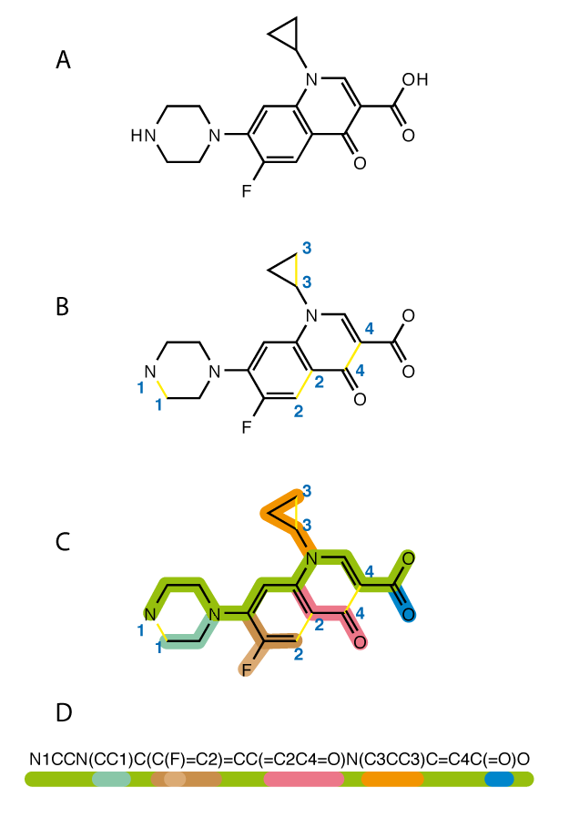
Before doing any drug parameterization we need to find a meaningful way to represent a drug, because drugs can be represented in several ways. We can draw the molecule or we can use text-based representations of the drugs like InChI or SMILES which are sequences of characters that represent the chemical structure of a molecule without losing information about it. That means that you can easily interconvert SMILES/InChI and drug drawings. Due to its simplicity compared with InChI I will use SMILES in the rest of the post.

Since most of the information about the drug is retained in the SMILES they are a very convenient way to encode, keep and trasfer information about a drug. You could for instance store millions of them in a USB stick. In later posts I will show you other interesting properties of the SMILES so they can be used in convolutional neural networks and/or in recursive neural networks.

Now that we know how to represent the drugs we need to find a way to parameterize them. Although there are several ways to do it, today I am just going to talk about the simplest of them: using chemical descriptors.

Chemical descriptors.

Chemical descriptors are numerical representations that cover different chemical properties of the drugs. There are hundreds of molecular descriptors that parametrize different features of the molecules, from the number of atoms or bonds to the solubility in water or the acdicity. By computing the chemical descriptors of a molecule we are predicting the physicochemical, topological, electronic and quantum properties of it and I say “predicting” because chemical descriptors of the molecule are calculated algorithmically, that means that some of them such as logP, logD or logS are just (very precise) predictions.

Ok. We have found a simple way to parametrize a drug by defining it as a vector of chemical descriptors that we could use to predicit its bioactivity.

The hypothesis is simple: drugs with simmilar chemical descriptors will have simmilar activities. Let’s test the hypothesis out.

Chemical descriptors calculation.

First of all, we need a dataset to test our hypothesis. In this case, I will use a dataset of molecules downloaded from ZINC15, which is a massive database of known and unknown compounds.

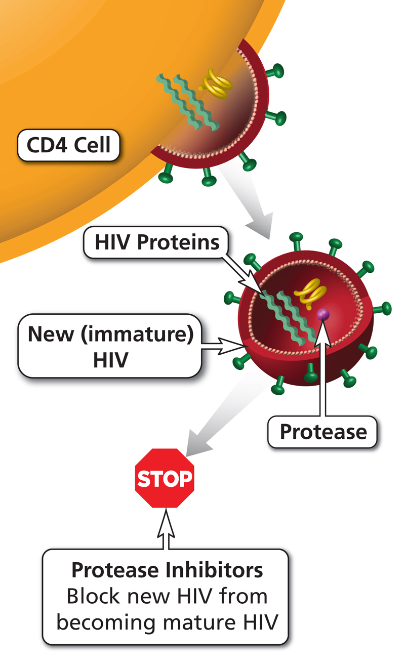
For this post, I have downloaded a set of 6102 molecules which are described to be proteases inhibitors. Proteases are enzymes that cut proteins. While some proteases have important biological roles for the physiology of the cell, others are essential for viruses to replicate and proteases inhibitors that specifically inhibit viral proteases are widely used as antivirals to treat HIV or Hepatitis C.
You can download the dataset yourself from ZINC15 or download it from here.

Once the file is ready we are going to load it into memory, but first let’s load the required libraries for the calculations (note that Rcpi needs to be installed through BioConductor and that if you are installing rcdk in Linux you will have to install rJava first)

library(Rcpi)
library(rcdk)
library(keras)
library(ggplot2)

and we load the paths where the training and test data are:

#Folders
path<-"C:/home/nacho/DrugDiscoveryWorkshop-master/SMILES_Activity.csv"
pathDB<-"/home/nacho/DrugDiscoveryWorkshop-master/ZINCDB/"

Next, we load the training set and we extract the chemical descriptors with the function extractDrugAIO.
Now you can go and get yourself a cup of coffee because this will take a while.

#Loading and descriptors calculation
df<-read.csv(path, sep = " ", header = FALSE)
df<-df[,c(1,5)]
df<-df[-1,]
colnames(df)<-c("SMILES","Affinity")
df$Affinity<-as.numeric(as.character(df$Affinity))
df<-df[complete.cases(df),]
mols <- sapply(as.character(df$SMILES), parse.smiles)
desc <- extractDrugAIO(mols,  silent=FALSE)

In order to save that time calculating the descriptors if you are considering playing around with the script, I recommend you to save the descriptors in a csv file that you can load each time you want to test something.

#Checkpoint
#write.csv(desc, "/home/nacho/StatisticalCodingClub/parameters.csv")
#desc<-read.csv("/home/nacho/StatisticalCodingClub/parameters.csv")

Now we need to clean up some of the variables. First, we remove those that contain NAs.

#Automatic cleaning
desc$X<-NULL
findNA<-apply(desc, 2, anyNA)
desc<-desc[,which(findNA==FALSE)]

Next, we clean those variables with the same value for all the drugs. We do it by calculating the standard deviation of the different variables. If the sd is zero, that means that all the values of the variable are the same so we can remove it.

findIdentical<- apply(desc, 2, sd)
desc<-desc[,which(findIdentical!=0)]

and finally, we manually clean some of the variables. In this case, I’ve found that some variables in the validation set only had one value so I removed them from the training set.

#Manual cleaning
to.remove<-c("ATSc1",
             "ATSc2",
             "ATSc3",
             "ATSc4",
             "ATSc5",
             "BCUTw.1l",
             "BCUTw.1h",
             "BCUTc.1l",
             "BCUTc.1h",
             "BCUTp.1l",
             "BCUTp.1h",
             "khs.tCH",
             "C2SP1")

`%!in%` = Negate(`%in%`)
desc<-desc[,which(names(desc) %!in% to.remove)]

Then, we standardize the values in the columns (the mean of the variables will be zero and the sd one) and we normalize the values of the activity so they range between zero and one:

x<-scale(desc)
y<-(df$Affinity-min(df$Affinity))/(max(df$Affinity)-min(df$Affinity))

Now it is time to prepare the training and validation datasets by dividing the dataset into training (90%) and validation (10%):

#Train/Test
val.ID<-sample(c(1:nrow(desc)),round(0.1*nrow(desc)))

x.val<-x[val.ID,]
y.val<-y[val.ID]
x<-x[-val.ID,]
y<-y[-val.ID]

For the model, I have just decided to create a very simple model with three fully-connected layers

We create the model with Keras/TensorFlow…

model<-keras_model_sequential()

model %>% layer_dense(units = 80, activation = "relu",  input_shape = (ncol(x))) %>% 
  layer_dense(units = 40, activation = "relu") %>% 
  layer_dense(units = 10, activation = "relu") %>% 
  layer_dense(units = 1, activation = "linear")
  

…compile it…

compile(model, optimizer = "adagrad", loss = "mean_absolute_error")

…and train it

history<-model %>% fit(x=x,
                       y=y,
                       validation_data=list(x.val, y.val),
                       callbacks = callback_tensorboard("logs/run_test"),
                       batch_size=5,
                       epochs=10
                        )
plot(history)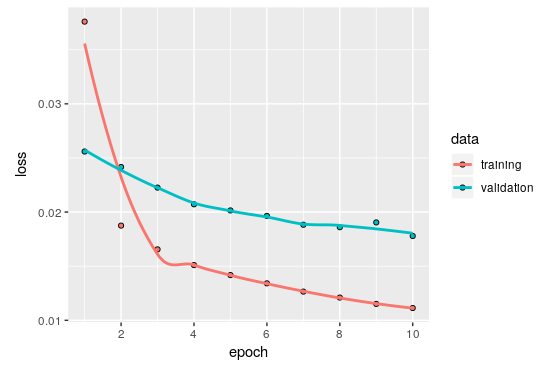

As you can see, the training went as expected and although it seems that it is not suffering from overfitting I decided to train only for 10 epochs.

Let’s see how well the model generalizes by trying to predict the activity of the validation set:

#Prediction over validation
y.hat<-predict(model, x.val)

ggplot()+
  geom_jitter(aes(x=y.val, y=y.hat), colour="red", size=2, alpha=0.5)+
  geom_smooth(aes(x=y.val, y=y.hat),method='lm',formula=y~x)+
  ylim(0,1)+
  xlab("Activity")+
  ylab("Predicted Activity")+
  theme_minimal()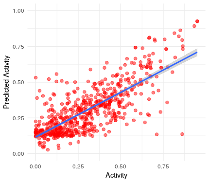

Wooow! Our first model is able to predict the activity of the drugs fairly well.
But let’s try to optimize it to see if there is a lot of space for improvement. To try to improve the model we are going to test different hyperparameters. In this case, we only modify the number of neurons and some activation functions while keeping the main architecture intact. In the following posts, I will show you how to modify the architecture of the model as another hyperparameter.

Briefly, we iterate over 200 models saving the hyperparameters in a dataframe and we test the mean square error for each model.

#Optimization
reset_states(model)
rounds<-200
models<-as.data.frame(matrix(data = NA, ncol =9 ,nrow = rounds))
colnames(models)<-c("UnitsL1", "UnitsL2", "UnitsL3", "act", "L1.norm", "L2.norm", "L1.norm.Rate", "L2.norm.Rate", "MSE")
pb<-txtProgressBar(min=1, max = rounds, initial = 1)

for (i in 1:rounds) {

  #Hyperparams
  unitsL1<-round(runif(1, min=20, max = 100))
  unitsL2<-round(runif(1, min=10, max = 60))
  unitsL3<-round(runif(1, min=2, max = 20))
  actlist<-c("tanh","sigmoid","relu","elu","selu")
  act<-actlist[round(runif(1,min = 1, max=5))]
  L1.norm<-round(runif(1,min = 0, max = 1))
  L2.norm<-round(runif(1,min = 0, max = 1))
  L1.norm.Rate<-runif(1, min = 0.1, max = 0.5)
  L2.norm.Rate<-runif(1, min = 0.1, max = 0.5)
  ###
  
  setTxtProgressBar(pb, i)
  model.search<-keras_model_sequential()
  
  model.search %>% layer_dense(units = unitsL1, activation = act, input_shape = (ncol(x)))
  if(L1.norm==1)  model.search %>% layer_dropout(rate=L1.norm.Rate)
  model.search %>% layer_dense(units = unitsL2, activation = act)
  if(L2.norm==1)  model.search %>% layer_dropout(rate=L2.norm.Rate)   
  model.search %>% layer_dense(units = unitsL3, activation = act) %>% 
  layer_dense(units = 1, activation = "sigmoid")
  
  compile(model.search, optimizer = "adagrad", loss = "mean_squared_error")
  model.search %>% fit(x=x,
                         y=y,
                         verbose=0,
                         batch_size=10,
                         epochs=10
  )
  
  y.hat<-predict(model.search, x.val)
  MSE<-(sum((y.val-y.hat)^2))/length(y.val)
  
  #FIlling dataframe
  models$MSE[i]<-MSE
  models$act[i]<-act
  models$UnitsL1[i]<-unitsL1
  models$UnitsL2[i]<-unitsL2
  models$UnitsL3[i]<-unitsL3
  models$L1.norm[i]<-L1.norm
  models$L2.norm[i]<-L2.norm
  models$L1.norm.Rate[i]<-L1.norm.Rate
  models$L2.norm.Rate[i]<-L2.norm.Rate
  reset_states(model.search)
  }
  

Next, we select the best set of hyperparameters to train a model to predict the activity of the test dataset:

#Validation best performer
models<-models[complete.cases(models),]
unitsL1<- models$UnitsL1[models$MSE==min(models$MSE)]
unitsL2<- models$UnitsL2[models$MSE==min(models$MSE)]
unitsL3<- models$UnitsL3[models$MSE==min(models$MSE)]

act<-models$act[models$MSE==min(models$MSE)]
L1.norm<-models$L1.norm[models$MSE==min(models$MSE)]
L2.norm<-models$L2.norm[models$MSE==min(models$MSE)]
L1.norm.Rate<-models$L1.norm.Rate[models$MSE==min(models$MSE)]
L2.norm.Rate<-models$L2.norm.Rate[models$MSE==min(models$MSE)]

model.best<-keras_model_sequential()

model.best %>% layer_dense(units = unitsL1, activation = act, input_shape = (ncol(x)))
if(L1.norm==1)  model.best %>% layer_dropout(rate=L1.norm.Rate)
model.best %>% layer_dense(units = unitsL2, activation = act)
if(L2.norm==1)  model.best %>% layer_dropout(rate=L2.norm.Rate)   
model.best %>% layer_dense(units = unitsL3, activation = act) %>% 
  layer_dense(units = 1, activation = act)

compile(model.best, optimizer = "adam", loss = "mean_squared_error")
model.best %>% fit(x=x,
                     y=y,
                     
                     batch_size=10,
                     epochs=10
)

y.hat<-predict(model.best, x.val)

ggplot()+
  geom_jitter(aes(x=y.val, y=y.hat), colour="red", size=2, alpha=0.5)+
  geom_smooth(aes(x=y.val, y=y.hat),method='lm',formula=y~x)+
  ylim(0,1)+
  xlab("Activity")+
  ylab("Predicted Activity")+
  theme_minimal()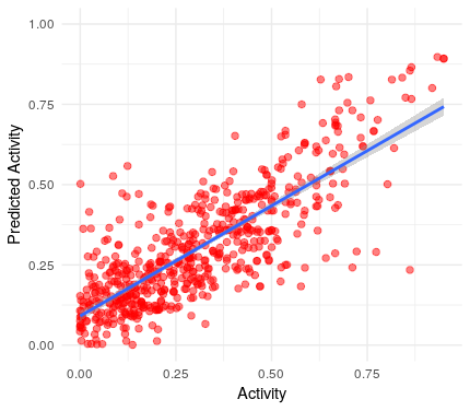

As you can see although the difference is not huge, meaning that we had proposed a good model as starting point, there is already a substantial improvement from the original model.

Then we save the model so we can reuse it or share it. Indeed you can download my trained model here.

save_model_hdf5(model.best, "/home/nacho/Drugs/BestModelNN.h5")
#model.best<-load_model_hdf5("/home/nacho/Drugs/BestModelNN.h5")

Now we are ready to find new protease-inhibitors among large libraries.

Since the next chunk of code contains a big while loop that I don’t want to cut, I will explain how it works here:

First, we define the folder in which the SMILES are. Next, we check that the files containing the SMILES have not been processed yet. This part is very useful because it allows you to add more files to the folder while the script is running so it keeps going iterating over the new files. Then, in order to avoid running out of memory when we process the SMILES, we load them in batches of 10000. To be able to normalize the data in the test set we need to use an additional function. This is because of the way the normalization step is done:

The normalization works only if we assume that our training and validation sets have the same mean and standard deviation, but that is simply not true in most of the cases. I solved this issue by using the mean and standard deviation of the training set to standardize the test set like this:

and this is exactly what the function scale.db does:

#Standarize based on previous data
scale.db<-function(df.new, df.old){
  if(ncol(df.new)!=ncol(df.old)) print("Error number of columns!")
  for (i in 1:ncol(df.new)) {
    df.new[,i]<- (df.new[,i]-mean(df.old[,i]))/sd(df.old[,i])
  }
  return(as.matrix(df.new))
}

Once the descriptors are extracted from the SMILES and the test is standardized we can proceed to predict the affinity of the drugs for the proteases.

Finally, we save the results in the disk every 1000 compounds and at the end of the process. Here is the code to do everything:

#Screening
db.completed<-vector()
db<-list.files(pathDB)
db.toprocess<-setdiff(db,db.completed)
if(length(db.toprocess>0)) continue=TRUE

while (continue) {

  batchsize<-10000
  batch.vector<-c(1,batchsize)
  
  smi.db<-read.csv(paste(pathDB,db.toprocess[1],sep=""), sep = " ", head=FALSE)
  db.completed[length(db.completed)+1]<-db.toprocess[1]

while(nrow(smi.db)>batch.vector[2]){
  mols.db <- sapply(as.character(smi.db$V1[batch.vector[1]:batch.vector[2]]), parse.smiles)  
  descs.db <- extractDrugAIO(mols.db,  silent=FALSE)
  findNA<-apply(descs.db, 2, anyNA)
  descs.db<-descs.db[,which(findNA==FALSE)]
  descs.db$khs.tCH<-NULL
  desc.db$C2SP1<-NULL
  desc.in.model<-colnames(desc)
  descs.db<-descs.db[,which(names(descs.db) %in% desc.in.model)]
  
  descs.db<-scale.db(descs.db,desc)

  predicted.act<-predict(model.best, descs.db)
  
  if(!exists("activity.db")) 
   {activity.db<- predicted.act}
  else{ activity.db<-c(activity.db, predicted.act)}
  
  batch.vector[1]<-sum(batch.vector)
  batch.vector[2]<-batch.vector[2]+batchsize
  if(batch.vector[2]>nrow(smi.db)) batch.vector[2]<-nrow(smi.db)
  
}

if(!exists("compound.db")) 
{compound.db<- smi.db$V2}
else{ compound.db<-c(compound.db, smi.db$V2)}   
  
db.toprocess<-setdiff(db,db.completed)  
if(length(db.toprocess==0)) continue==FALSE  
counter<-counter+1  
if(counter%%1000=0){
  output<-data.frame(compound.db,activity.db) 
  write.csv(output,paste(pathDB,"results.csv",sep = ""))
  }

} 

output<-data.frame(compound.db,activity.db)
write.csv(output,paste(pathDB,"results.csv",sep = ""))

And this is it.
Now you have the tools to start your own search for bioactive drugs.

Conclusions

In this post, I have shown you the very basics of drug discovery so you can get an intuition about how using ML approaches can speed up the search for new medicines.
Even though I have shown you how to extract and use chemical descriptors in most of the cases this is not a good idea, the reason for that is that during the extraction of the descriptors there is a huge loss of information. In the next post, I will explain how to use convolutional neural networks to increase the efficacy of the drug-discovery process by using lossless parametrizations of the drugs. Anyway, I hope you have enjoyed it.

As always, you can download my code from here and a pdf that I prepared for a workshop about this topic here.

Sources of images

SMILES
Protease inhibitors Chemical representations