
Teaching a Computer How to Draw
Do Androids Dream of Electric Sheep? Let’s talk about VAAAAAAAAAAAAAAAEs!!!
Introduction
My son’s favorite animal is sheep. He still doesn’t talk and he doesn’t know the name of the animal, but he bleats each time he sees one, it doesn’t matter if it is in a book, a video, a plastic figure or in real life. He clearly knows how a sheep looks like.
I know that I have already discussed this kind of topics before but I would like to bring this question up again because the more I understand how difficult is to train machines the more I realize how amazing the human brain is.
With just one year, the developing human brain has all the neuronal circuits that allow it to learn to recognize patterns no matter how different they are. Think for a second how different it is to see a sheep in the fields when compared with a more or less accurate drawn of a sheep in a book.
But not only that, a human brain has stored the idea of how a sheep looks like and it can extract that encoded information to draw a sheep anytime.
In this post, we will see how to train a computer to do exactly the same, recognize, store and draw a picture of a sheep.
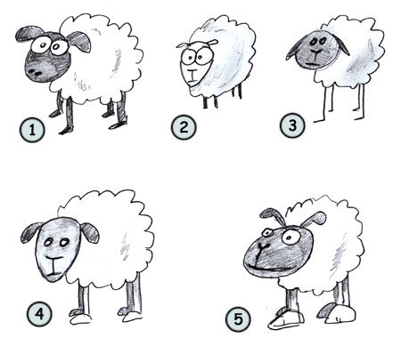
Image taken from here
VAEs again and bit more of the theory
Although in a previous post I already talked about VAEs and how to use them, I would like to review that type of models a bit further.
VAEs are models that rely on the idea that it is possible to create a low-dimensional representation of the input data. This representation is usually called latent space and VAE’s theory proposes that by sampling this latent space, it is possible to create new items similar to the ones presented to the model during the training process.
Let’s translate this idea to the sheep example: If you ask someone to draw a sheep, that person could draw not one but one thousand different sheep still recognizable as sheep and the mechanisms involved in those processes are not very different from VAEs since they rely on specific low-dimension neuronal circuitry used to store information about how sheep look like. That is the biological latent space of the human brain.
To train a computer to do something similar we need an algorithm able to encode the parameters necessary to draw a sheep. Although these parameters can be N-dimensional vectors, it is very common for these vectors to have only two dimensions. The distribution of all possible vectors for all possible sheep laying in this latent space integrates the sheep-allowed latent space. All vectors representing a sheep lay there and all vectors representing something else lay somewhere else in the latent space and that is why the representation of vectors in the latent space can be studied as a probabilistic problem.
The probability of drawing a sheep P(X) can be enlarged by increasing two factors: The probability of selecting an area of the latent space that belongs to the sheep-allowed region P(z) and the probability of actually drawing a sheep if we select a vector from that sheep-allowed region P(X|z):
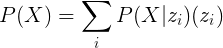
And this is exactly what a VAE does: It increases the P(z) by constraining it and it increases P(X|z) by reducing the differences between inputs and predictions during the training. All this is achieved by using a custom loss function with two terms, one to maximize P(z) and other to maximize P(X|z).
The first thing that it’s probably popping into your mind after reading this is “How can you increase P(z) by constraining it?” Well… imagine that you are in the shooting range and that you have nine targets of 10cm by 10cm. What is it easier? To hit one of the nine 10x10 targets or to hit just one 30x30 target? You increase the probability of hitting a target by constraining the region where the targets can be. If you are curious abut the statistical details click here.
The sheep dataset
Now that we are done with the theory, we can start obtaining the sheep. For this project we are going to use a dataset with thousands of hand-drawn sheep from Google’s Quickdraw game from here. If you visit the link you will find that it is possible to get the dataset in different file formats and we are going to use one of them, the .npy format.
.npy is a Python-specific format, so in order to load the files into R you need to import the Python numpy library first. We do that using the R library reticulate.
Next, you have to reshape the array so it has the shape {number-of-samples, 28, 28}.
Then we normalize the values by dividing them by 255 and we save a copy of the files in .csv, a more R-friendly format.
Finally, it is important to unload the reticulate package otherwise Keras doesn’t work.
Here is the code to do everything:
library(reticulate)
 np <- import("numpy")

 df<-np$load("/home/nacho/VAE_Faces/full_numpy_bitmap_sheep.npy")
 df<-array(df, dim = c(dim(df)[1], 28,28)) #Reshape
 df<-df/255 #Normalization
 write.csv(df, "/home/nacho/VAE_Faces/datasheep.csv") #Checkpoint

 detach("package:reticulate", unload=TRUE)
If you have saved the images as .csv you don’t need to run this part each time you play around with the dataset, you just load the .csv, from the checkpoint.
library(keras)
library(imager)
library(ggplot2)

df<-read.csv("/home/nacho/VAE_Faces/datasheep.csv")
df<-as.matrix(df)
df<-array(as.numeric(df[,2:785]), dim = c(nrow(df),28,28,1))
Next, you load the images and you reshape the array to the shape {number-of-samples,28,28,1}, the last dimension is 1 because there is only one channel, black and white.
The encoder
Now that the data is ready, we can start creating the encoder part of the model which is indeed very similar to the one that I described here and that it is actually an adapted version of this one.
The encoder consists of a set of convolutional layers to capture the features of the drawings, these layers are then connected to a neural net to model the possible non-linear relationships of the features:
#Model
reset_states(vae)
filters <- 10
intermediate_dim<-100
latent_dim<-2
epsilon_std <- 1
batch_size <- 8
epoch<-15
activation<-"relu"

dimensions<-dim(df)
dimensions<-dimensions[-1]

Input <- layer_input(shape = dimensions)

faces<- Input %>%
  layer_conv_2d(filters=filters, kernel_size=c(4,4), activation=activation,
  padding='same',strides=c(1,1),data_format='channels_last')%>%
  layer_conv_2d(filters=filters*2, kernel_size=c(4,4), activation=activation,
  padding='same',strides=c(1,1),data_format='channels_last')%>%
  layer_conv_2d(filters=filters*4, kernel_size=c(4,4), activation=activation,
  padding='same',strides=c(1,1),data_format='channels_last')%>%
  layer_conv_2d(filters=filters*8, kernel_size=c(4,4), activation=activation,
  padding='same',strides=c(1,1),data_format='channels_last')%>%
  layer_flatten()

hidden <- faces %>% layer_dense( units = intermediate_dim,
activation = activation) %>%
  layer_dropout(0.1) %>%
  layer_batch_normalization() %>%
  layer_dense( units = round(intermediate_dim/2), activation = activation) %>%
  layer_dropout(0.1) %>%
  layer_batch_normalization() %>%
  layer_dense( units = round(intermediate_dim/4), activation = activation)
The latent space
The latent space is created using a lambda layer. Lambda layers in Keras are custom layers that are used to wrap functions. In our case, we create two additional layers z_mean and z_log_var that we concatenate and transform using the sampling function.
z_mean <- hidden %>% layer_dense( units = latent_dim)
z_log_var <- hidden %>% layer_dense( units = latent_dim)


sampling <- function(args) {
  z_mean <- args[, 1:(latent_dim)]
  z_log_var <- args[, (latent_dim + 1):(2 * latent_dim)]

  epsilon <- k_random_normal(
    shape = c(k_shape(z_mean)[[1]]),
    mean = 0.,
    stddev = epsilon_std
  )
  z_mean + k_exp(z_log_var) * epsilon
}

z <- layer_concatenate(list(z_mean, z_log_var)) %>%
layer_lambda(sampling, name="LatentSpace")
The decoder
Now we need to write the decoder part of the VAE in a way that we can use it also to sample the latent space. To do this we need to share the layers between two models: the end-to-end VAE and the decoder itself, that is why this part might look a bit unusual if you compare it with the encoder. The reason for that is that we initialize all layers independently to be able to share them with their weights after training the model.
Another way of doind this would be creating two independent models with the same architecture and transfering the weights from the trained end-to-end VAE to the decoder.
Here is the code to do this. We initialize the layers one by one and then we bind them:
#Initialization of layers

Output1<- layer_dense( units = round(intermediate_dim/4), activation = activation)
Output2<- layer_dropout(rate=0.1)
Output3<- layer_batch_normalization()
Output4<- layer_dense( units = round(intermediate_dim/2), activation = activation)
Output5<- layer_dense(units = intermediate_dim, activation = activation)
Output6<- layer_dense(units = prod(28,28,filters*8), activation = activation)
Output7<- layer_reshape(target_shape = c(28,28,filters*8))
Output8<- layer_conv_2d_transpose(filters=filters*8, kernel_size=c(4,4), activation=activation,
 padding='same',strides=c(1,1),data_format='channels_last')
Output9<- layer_conv_2d_transpose(filters=filters*4, kernel_size=c(4,4), activation=activation,
 padding='same',strides=c(1,1),data_format='channels_last')
Output10<-layer_conv_2d_transpose(filters=filters*2, kernel_size=c(4,4), activation=activation,
 padding='same',strides=c(1,1),data_format='channels_last')
Output11<-layer_conv_2d_transpose(filters=filters, kernel_size=c(4,4), activation=activation,
 padding='same',strides=c(2,2),data_format='channels_last')
Output12<-layer_conv_2d(filters=1, kernel_size=c(4,4), activation="sigmoid",
 padding='same',strides=c(2,2),data_format='channels_last')

#Concatenation of layers for the VAE

O1<-Output1(z)
O2<-Output2(O1)
O3<-Output3(O2)
O4<-Output4(O3)
O5<-Output5(O4)
O6<-Output6(O5)
O7<-Output7(O6)
O8<-Output8(O7)
O9<-Output9(O8)
O10<-Output10(O9)
O11<-Output11(O10)
O12<-Output12(O11)

#Concatenation of layers for the Decoder

decoder_input <- layer_input(shape = latent_dim)
O1D<-Output1(decoder_input)
O2D<-Output2(O1D)
O3D<-Output3(O2D)
O4D<-Output4(O3D)
O5D<-Output5(O4D)
O6D<-Output6(O5D)
O7D<-Output7(O6D)
O8D<-Output8(O7D)
O9D<-Output9(O8D)
O10D<-Output10(O9D)
O11D<-Output11(O10D)
O12D<-Output12(O11D)
Now we can create the two models and get a summary of them:
## variational autoencoder
vae <- keras_model(Input, O12)
summary(vae)

#Decoder
decoder<- keras_model(decoder_input, O12D)
summary(decoder)
> summary(vae)
_________________________________________________________________________________________
Layer (type)                 Output Shape       Param #    Connected to
=========================================================================================
input_1 (InputLayer)         (None, 28, 28, 1)  0
_________________________________________________________________________________________
conv2d (Conv2D)              (None, 28, 28, 10) 170        input_1[0][0]
_________________________________________________________________________________________
conv2d_1 (Conv2D)            (None, 28, 28, 20) 3220       conv2d[0][0]
_________________________________________________________________________________________
conv2d_2 (Conv2D)            (None, 28, 28, 40) 12840      conv2d_1[0][0]
_________________________________________________________________________________________
conv2d_3 (Conv2D)            (None, 28, 28, 80) 51280      conv2d_2[0][0]
_________________________________________________________________________________________
flatten (Flatten)            (None, 62720)      0          conv2d_3[0][0]
_________________________________________________________________________________________
dense (Dense)                (None, 100)        6272100    flatten[0][0]
_________________________________________________________________________________________
dropout (Dropout)            (None, 100)        0          dense[0][0]
_________________________________________________________________________________________
batch_normalization_v1 (Batc (None, 100)        400        dropout[0][0]
_________________________________________________________________________________________
dense_1 (Dense)              (None, 50)         5050       batch_normalization_v1[0][0]
_________________________________________________________________________________________
dropout_1 (Dropout)          (None, 50)         0          dense_1[0][0]
_________________________________________________________________________________________
batch_normalization_v1_1 (Ba (None, 50)         200        dropout_1[0][0]
_________________________________________________________________________________________
dense_2 (Dense)              (None, 25)         1275       batch_normalization_v1_1[0][0]
_________________________________________________________________________________________
dense_3 (Dense)              (None, 2)          52         dense_2[0][0]
_________________________________________________________________________________________
dense_4 (Dense)              (None, 2)          52         dense_2[0][0]
_________________________________________________________________________________________
concatenate (Concatenate)    (None, 4)          0          dense_3[0][0]
                                                           dense_4[0][0]
_________________________________________________________________________________________
LatentSpace (Lambda)         (None, 2)          0          concatenate[0][0]
_________________________________________________________________________________________
dense_5 (Dense)              (None, 25)         75         LatentSpace[0][0]
_________________________________________________________________________________________
dropout_2 (Dropout)          (None, 25)         0          dense_5[2][0]
_________________________________________________________________________________________
batch_normalization_v1_2 (Ba (None, 25)         100        dropout_2[2][0]
_________________________________________________________________________________________
dense_6 (Dense)              (None, 50)         1300       batch_normalization_v1_2[2][0]
_________________________________________________________________________________________
dense_7 (Dense)              (None, 100)        5100       dense_6[2][0]
_________________________________________________________________________________________
dense_8 (Dense)              (None, 62720)      6334720    dense_7[2][0]
_________________________________________________________________________________________
reshape (Reshape)            (None, 28, 28, 80) 0          dense_8[2][0]
_________________________________________________________________________________________
conv2d_transpose (Conv2DTran (None, 28, 28, 80) 102480     reshape[2][0]
_________________________________________________________________________________________
conv2d_transpose_1 (Conv2DTr (None, 28, 28, 40) 51240      conv2d_transpose[2][0]
_________________________________________________________________________________________
conv2d_transpose_2 (Conv2DTr (None, 28, 28, 20) 12820      conv2d_transpose_1[2][0]
_________________________________________________________________________________________
conv2d_transpose_3 (Conv2DTr (None, 56, 56, 10) 3210       conv2d_transpose_2[2][0]
_________________________________________________________________________________________
conv2d_4 (Conv2D)            (None, 28, 28, 1)  161        conv2d_transpose_3[2][0]
=========================================================================================
Total params: 12,857,845
Trainable params: 12,857,495
Non-trainable params: 350
_________________________________________________________________________________________
> summary(decoder)
_________________________________________________________________________________________
Layer (type)                            Output Shape                       Param #
=========================================================================================
input_5 (InputLayer)                    (None, 2)                          0
_________________________________________________________________________________________
dense_5 (Dense)                         (None, 25)                         75
_________________________________________________________________________________________
dropout_2 (Dropout)                     (None, 25)                         0
_________________________________________________________________________________________
batch_normalization_v1_2 (BatchNormaliz (None, 25)                         100
_________________________________________________________________________________________
dense_6 (Dense)                         (None, 50)                         1300
_________________________________________________________________________________________
dense_7 (Dense)                         (None, 100)                        5100
_________________________________________________________________________________________
dense_8 (Dense)                         (None, 62720)                      6334720
_________________________________________________________________________________________
reshape (Reshape)                       (None, 28, 28, 80)                 0
_________________________________________________________________________________________
conv2d_transpose (Conv2DTranspose)      (None, 28, 28, 80)                 102480
_________________________________________________________________________________________
conv2d_transpose_1 (Conv2DTranspose)    (None, 28, 28, 40)                 51240
_________________________________________________________________________________________
conv2d_transpose_2 (Conv2DTranspose)    (None, 28, 28, 20)                 12820
_________________________________________________________________________________________
conv2d_transpose_3 (Conv2DTranspose)    (None, 56, 56, 10)                 3210
_________________________________________________________________________________________
conv2d_4 (Conv2D)                       (None, 28, 28, 1)                  161
=========================================================================================
Total params: 6,511,206
Trainable params: 6,511,156
Non-trainable params: 50
_________________________________________________________________________________________
KL-Anneling
Now that we have created the models, we are ready for the next step which is to create the custom loss function, but before we do it I would like to introduce an additional concept, the Kullback-Leibler annealing (KL-Annealing).
As I mentioned previously, the loss function is the result of assembling two sub-loss functions: The mean squared error (MSE) that accounts for the fidelity of the model and the Kullback-Leibler divergence (KL-Divergence) that constrains the distribution of samples in the latent space; however, these two terms are partially opposing each other and under some circumstances (e.g. noisy input, high input variance) the trained model falls into a local minima called posterior collapse. When this happens the model learns to avoid the latent space so all the samples have the same values for the latent variables. I have personally experienced it when training models for the generation of faces and it is impossible to generate any sample if that happens.
Fortunately for us, there are several solutions to prevent the posterior collapse and one of them is the so called KL-Annealing.
The KL-Annealing consists in the introduction of a weight to control the KL-Divergence during the training in a way that we train the model for some epochs just using the MSE and after certain epoch, we start to increase slowly the weight of the KL-Divergence to reach its maximun after few epochs.
Implementing KL-Annealing means that we need to modify the loss function dynamically during the training. This can be done in Keras/Tensoflow by using callbacks. Callbacks allow us to modify some parameters of the training process while it is happening. Unfortunately, the documentation to do that in Python is pretty sparse and in R it’s just negligible. So if you are interested in knowing how to write callbacks for Keras in R keep reading.
First we need to create a class-like element in R using the R6 package
#Custom callback KL-Annealing

KL.Ann <- R6::R6Class("KL.Ann",
#We create a KerasCallback-like class by inheriting the shape
                      inherit = KerasCallback,

                      public = list(
#Here we define and assingn the variables that we are going to use in the class (weight)

                        losses = NULL,
                        params = NULL,
                        model = NULL,
                        weight = NULL,

                        set_context = function(params = NULL, model = NULL) {
                          self$params <- params
                          self$model <- model
                          self$weight<-weight
                        },
#Here we define a function that runs at the end of each epoch
#We modify the weight value according to three parameters
#Epoch: The current epoch
#kl.start: The last epoch in which the KL weight is 0
#kl.steep: The length in epochs of the KL increase

                        on_epoch_end = function(epoch, logs = NULL) {

                          if(epoch>kl.start){
                            new_weight<- min((epoch-kl.start)/kl.steep,1)
                            k_set_value(self$weight, new_weight)
                            print(paste("     ANNEALING KLD:", k_get_value(self$weight), sep = " "))

                          }
                        }

                      ))
and then we define the variables to be used during KL-Annealing.
#Starting weight = 0
weight <- k_variable(0)
epochs <-30
kl.start <-10
kl.steep <- 10weight(sic) is how much of the KL-Divergence we put at the beginning of the training process, epochs is for how many epochs we run the training, kl.start is the epoch number in which we start increasing the KL-Divergence and kl.steep is the number of epochs that last the increase. In our case it means that the maximum KL-Divergence will be achieved at epoch 20.
The loss function
Now we are really ready to create the custom loss function. The loss function will consist of an external function wrapping a proper loss function (l.f in the code). I say proper because it is the one that compares Y and Ŷ. The wrapping function just takes the parameter weight and passes it to l.f before returning the function.
loss<- function(weight){
  l.f<-function(x, x_decoded_mean){

    x <- k_flatten(x)
    x_decoded_mean <- k_flatten(x_decoded_mean)
    xent_loss <- 2.0 * dimensions[1]* dimensions[2]*loss_mean_squared_error(x, x_decoded_mean)
    kl_loss <- -0.5*k_mean(1 + z_log_var - k_square(z_mean) - k_exp(z_log_var), axis = -1L)
    xent_loss + weight*kl_loss}
  return(l.f)
}
Now we can compile the model and start the training process:
vae %>% compile(optimizer = "rmsprop", loss = loss(weight))Setting up the GPU to be used by Keras in R
Before describing the training process I would like to briefly outline the process of setting up the GPU of the computer instead of the CPU for training purposes.
First. Why should you train on your GPU instead of on your CPU? Mainly because of speed, even if you have a decent CPU (an Intel i7-8700 with 12 threads) a normal GPU (an NVIDIA GTX1060 embedded on a laptop) trains the very same model 15 times faster.
How do you do it? I have to tell you that it is not so trivial to do set up the GPU for training ML models in R and again the documentation is pretty sparse. The main (and almost sole) guidelines are these.
Briefly, you have to download an install the CUDA Toolkit and the cuDNN libraries. It is VERY IMPORTANT that you download the proper versions of each library. In the guidelines they say that you need to download the CUDA Toolkit v9 and the cuDNN v7.0 but the truth is that those versions are a bit outdated so you can use more recent versions of the libraries, the problem is that not all versions are compatible among them and with TensorFlow.
After several trial and error tests I have found an optimal combination of settings:
CUDA Toolkit: Cuda compilation tools, release 10.0, V10.0.130
cuDNN: 7.4.2
Tensorflow: 1.13
To install them you need to follow the instructions provided in the link above and you shouldn’t get any problem. In case that by the time you read these lines there are new versions of the libraries, remember that it is essential to check the cross-compatiblity before doing any installation.
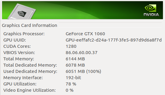
This is a picture of my NVIDIA panel during training: 61ºC at 78% of its capacity.
Training the model
Now we are all set for the training of the model.
date<-as.character(date())
logs<-gsub(" ","_",date)
logs<-gsub(":",".",logs)
logs<-paste("logs/",logs,sep = "")

#Callbcks
tb<-callback_tensorboard(logs)
anneling <- KL.Ann$new()

history<-vae %>% fit(x= df,
                y= df,
                batch_size=batch_size,
                epoch=epochs,
                callbacks = list(tb,annealing),
                view_metrics=FALSE,
                shuffle=TRUE)
We can visualize the training process using tensorboard:
tensorboard(logs)We can also save the weights to avoid doing the training each time you run the script.
save_model_weights_hdf5(vae, "/home/nacho/VAE_Faces/Baeh.h5")if you save the weights you can load them back into your model by doing this:
load_model_weights_hdf5(vae, "/home/nacho/VAE_Faces/Baeh.h5")This is how the training process looks like:
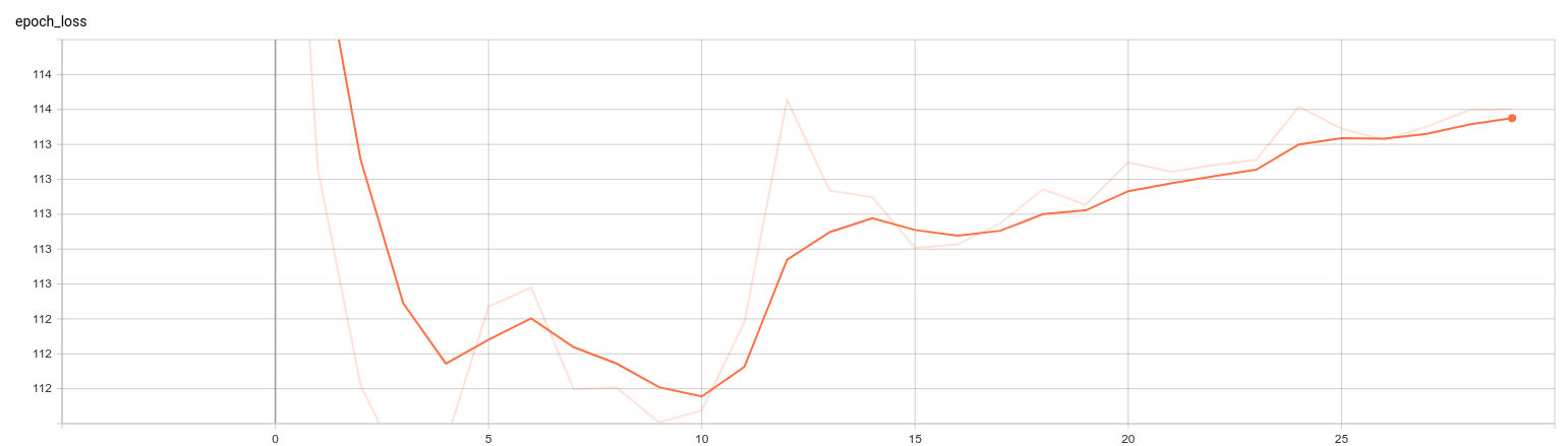
As you can see, as soon as we start introducing the KL-Divergence at epoch 10 the total loss increases (as expected, remember that I told you that those two terms oppose each other, at least partially) but it seems that in general the model handles it well because the increase doesn’t get out of range.
Exploring the latent space
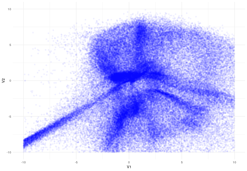
The next think that I would like to show you how the latent space changes when the KL divergence is applied:
Latent Space after 5 epocs (I did the training only in 10.000 samples for simplicity)
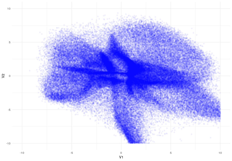
Latent Space after 10 epocs
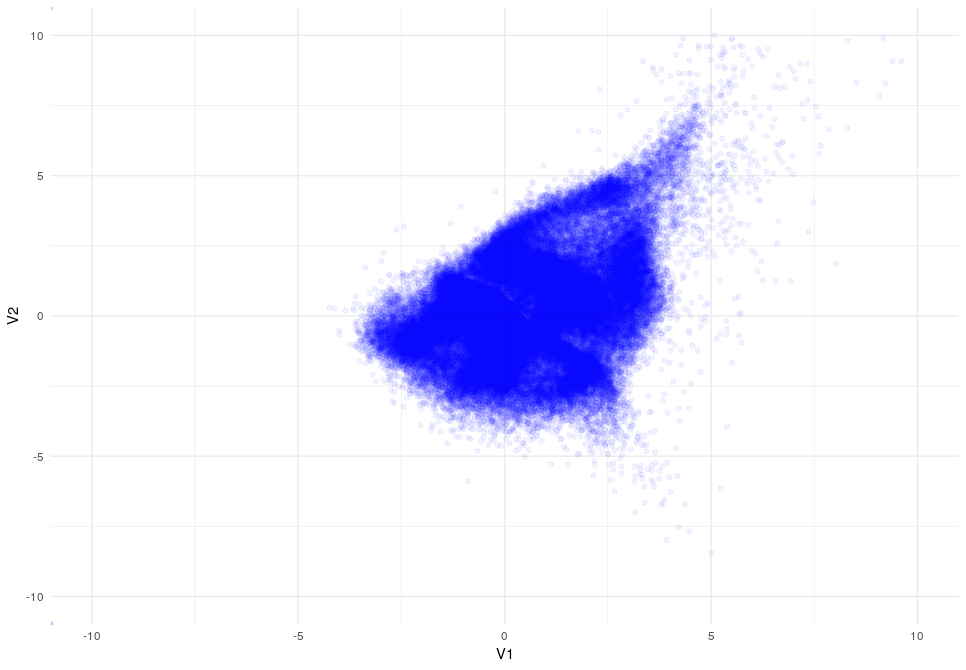
Latent Space after 15 epocs
Latent Space after 20 epocs
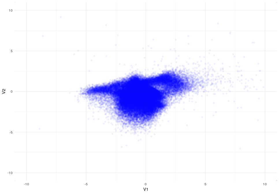
As you can appreciate the introduction of the KL-Divergence does its job very well modifying the latent space by constraining the data.
K-means
Interestingly, we can observe some patterns in the latent space despite the effect of the KL-Divergence. The presence of patterns suggests the existence of different classes of drawings, so let’s try to explore them further.
First of all, we can try to find the clusters in the dataset using k-means. K-means is a very powerful algorithm that usually is strong enough to do the job of finding clusters (you can check how I use k-means to predict human populations based on genetic information here). Unfortunately, in this case, k-means does not work. It is impossible to find out the optimal number of clusters by using the Elbow method as it is commonly done.
This is how the plot for the Elbow method looks like after 20 epochs (note that there is no curve to estimate the k)
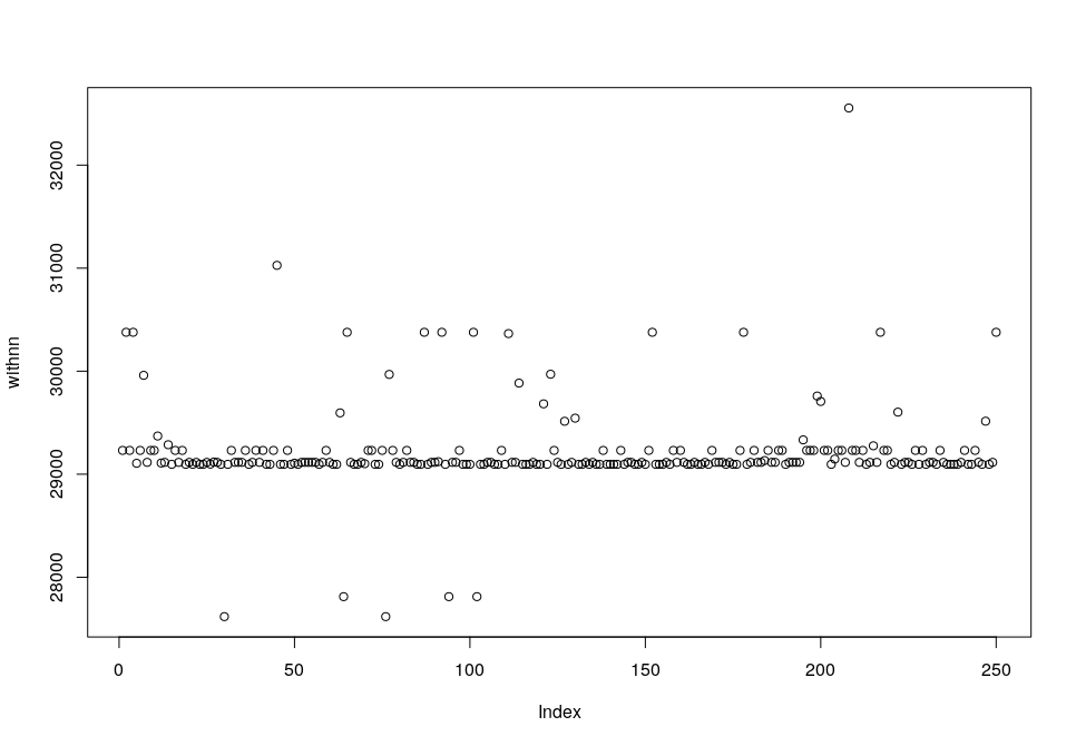
And this is how clusters are distributed when k=100.
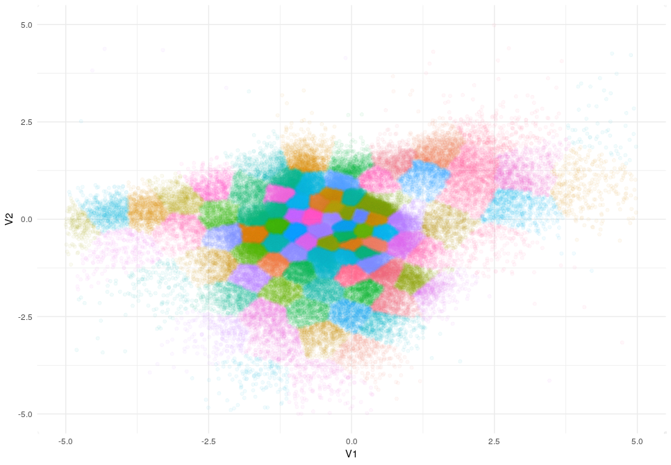
Clusters distribute as a mosaic without following any clear pattern. So we definitely need a better method and this is when DBSCAN comes in.
DBSCAN
DBSCAN as k-means is an unsupervised algorithm used in machine learning, but one of the main differences with k-means is that DBSCAN is very good at finding patterns and this is exactly what we want.
On the other hand, the downside of the algorithm is that it is more difficult to tune. While in k-means the only relevant parameter is the number of clusters (K) and it is very intuitive to understand its meaning. DBSCAN clustering needs two parameters MinPoint: The minimal number of points to be considered as a cluster and Epsilon: The distance between two points to be considered as part of the same cluster. Although the definitions of both parameters seem to easily interpretable, usually it is not that obvious to estimate them and sometimes they need to be tuned by trial and error.
Note that there is an analogous method to the Elbow method for k-means using the function kNNdistplot but it fails in the same way as the Elbow method does in our latent space. So the only solution is to perform a random search for the hyperparameters Epsilon, and MinPoint.
db<-as.data.frame(matrix(data = NA, ncol = 3, nrow = 100))

pb<-txtProgressBar(min = 1, max = 100, initial = 1)
for (i in 1:100) {
  setTxtProgressBar(pb,i)
  eps<-runif(1, min = 0.005, max =0.5 )
  mp<-round(runif(1,min = 5, max = 300))
  dummy<-dbscan(intermediate_output[-to.remove,1:2], eps = eps, MinPts = mp)
  db[i,1]<-eps
  db[i,2]<-mp
  db[i,3]<-max(dummy$cluster)
}
After 100 iterations we look for the parameters that give us a reasonable number of clusters (saved in db[,3]) and assign clusters according to them.
dbs<-dbscan(intermediate_output[-to.remove,1:2], eps = 0.04270631, MinPts = 377)
intermediate_output[-to.remove,]$Cluster<-dbs$cluster
These parameters give us eight clusters that look like this:
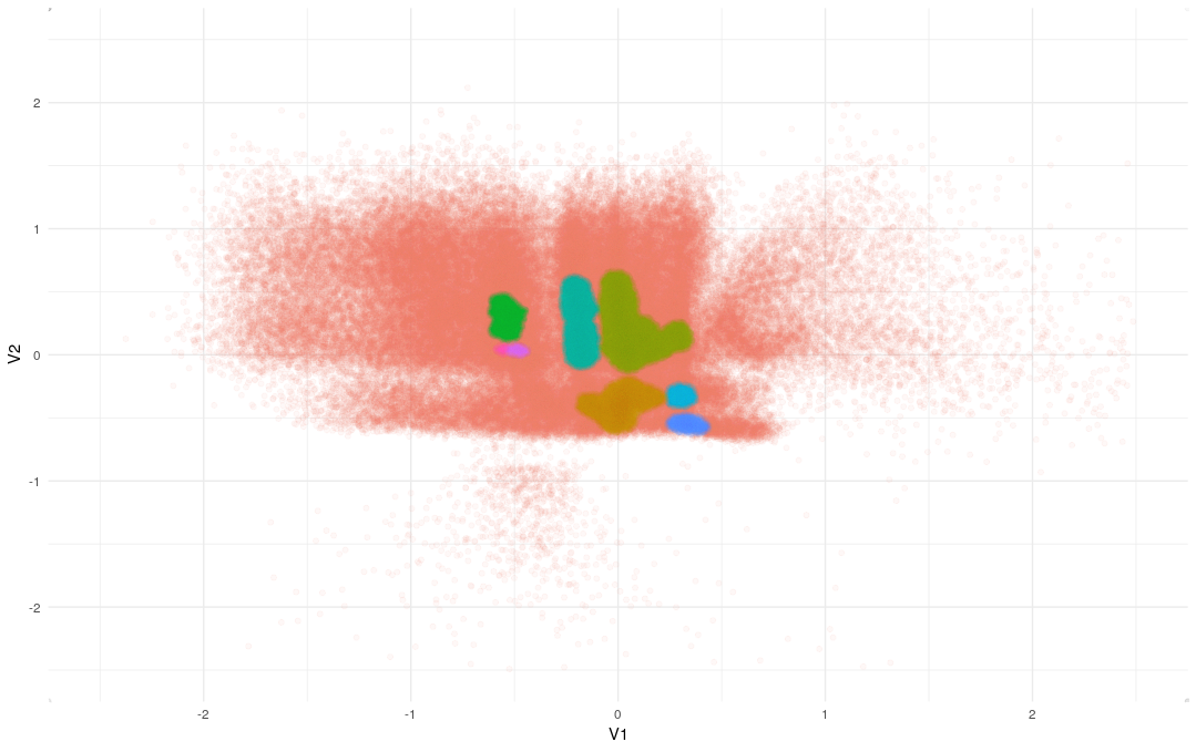
The hypothesis now is that the different clusters will group different representations of sheep so let’s explore some of the images that fall into each cluster to validate the hypothesis.
To plot some images of clusters 3 (green) and 6 (blue) we use this code:
cluster6<-which(intermediate_output$Cluster==6)
cluster8<-which(intermediate_output$Cluster==8)

sample6<-df[sample(cluster6,1),,,]
sample8<-df[sample(cluster8,1),,,]

cbind(abs(sample6-1),abs(sample8-1)) %>% as.raster() %>% plot()
That gives us this output after running it three times:
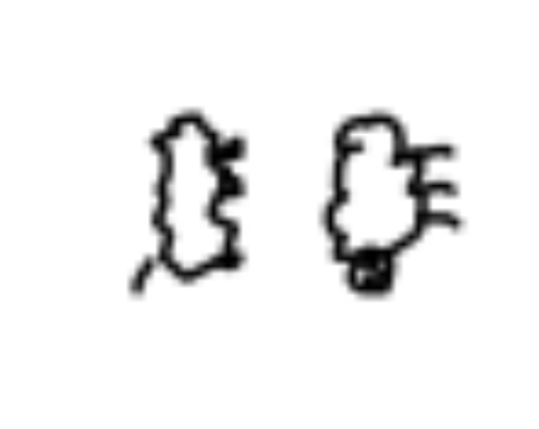
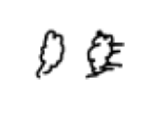
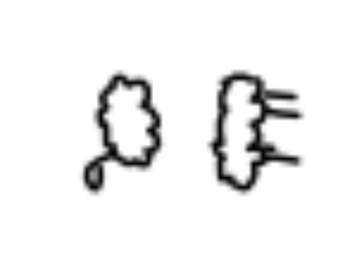
It looks like most of the sheep in cluster six don’t have legs (or they are small) while sheep in cluster eight do have prominent legs.
As you can appreciate the use of unsupervised learning strategies give us a lot of information about the samples that we are studying and that brings me to the next point.
Annomaly detection
As I have shown you, we can use the latent space to cluster and disect the samples. Now, we will use the predictions of an autoencoder as a tool to detect anomalies.
Let’s say that someone dropped some drawings of cars among the drawings of sheep. How could we find them?
Easy, we create an autoencoder and then we find which samples have a higher MSE when they are sent through the model. Since the model has learned how sheep look like the more a sample deviate from a sheep the higher the MSE of that sample will be.
Let’s apply this strategy to our sheep-dataset:
#Annomaly detection
MSE<-vector()
pb<-txtProgressBar(min = 1, max = 100, initial = 1)
for (i in 1:ncol(df)) {
  setTxtProgressBar(pb,i)
  dummy<-predict(vae, df[i,,,,drop=FALSE], batch_size = 10)
  MSE[i] <- sum((df[i,,,] - dummy[1,,,])^2)
}
plot(MSE)
Then, we stablish a cut-off to classify a sample as annomalous
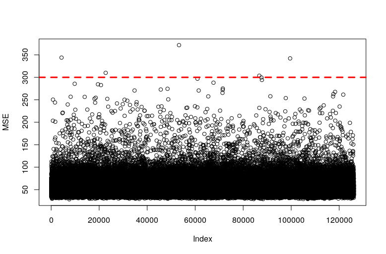
and we retreive the samples with higher MSE than our cut-off
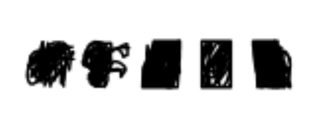
It seems very clear that we have found anomalies. Some drawings are just not sheep and the one that resembles a sheep is indeed a black sheep, which is usually the common definition of anomalous sheep.
Generation of new pictures
So far we have seen how to create a model to capture information about drawing of sheep based on thousands of pictures. We have seen how that the model can learn features like the possibility of drawing sheep with or without legs and it can even discriminate black sheep.
But now we are going to see something more interesting and funnier I will show you how this model can create new drawings of sheep, similar to the ones in the data set but at the same time different from all of them.
For this part, we are going to use the decoder model that we created before. As the decoder has shared layers with the end-to-end model, the trained weights are ready, we only need to provide a 2D vector representing a position in the latent space and the decoder will draw a sheep for us.
Let’s try it out selecting vectors belonging to a couple of different areas (cluster three and cluster six)
# generator, from latent space to reconstructed inputs

Samp<-array(data = c(rnorm(1, mean = 1, sd=0.5),rnorm(1, mean = 1, sd=0.5)), dim = c(1,2))
Samp<- predict(decoder, generator.arrray, batch_size = 10)
Samp <- Samp[1,,,1]

for (i in 1:2) {
  generator.arrray<-array(data = c(rnorm(1, mean = 1, sd=0.5),rnorm(1, mean = 1, sd=0.5)), dim = c(1,2))
  Gen1 <- predict(decoder, generator.arrray, batch_size = 10)
  Gen1 <- Gen1[1,,,1]
  Samp<-cbind(Samp,Gen1)

}
abs(Samp-1) %>% as.raster() %>% plot()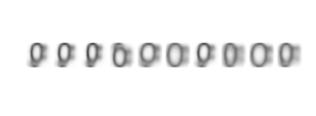
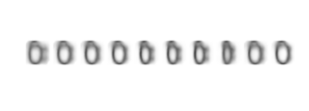
Amazing!!, the model not only recognize sheep with or withoug legs, it has also learned how to draw them!!!.

You might think that the drawings are not very good, but they are way better than some of the ones that are included in the dataset and indeed they clearly could be clasified as sheep.
You have to consider also that we have only trained for 30 epochs and a that latent space has only two dimensions so the margin to improve very still broad.
If you want to take it from here and enhance it, you should probably start by doing an hyperparameter search for different architectures (including a 3D/4D latent space).
And of course, feel free to use my code that you can download from here
Conclusions
In this post I have shown you how to create and train a model to draw sheeps, how to create callbacks in R, how to use the GPU for training and how to do unsupervised learning to find clusters and anomalies and more interestingly I have shown you how much you can learn and how much fun you can get just playing with simple data-sets.
See you next post…