Introduction

December the 31st, the Chinese health authorities reported a case of pneumonia of unknown origin. On January the 3rd, another 43 cases were reported to the WHO. Twelve days later, the Chinese government had found that all the cases of pneumonia were caused by a new type of coronavirus and traced back the origin of the disease to a seafood market in Wuhan.
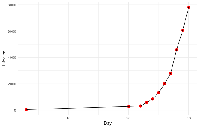
One month later Wuhan is under lockdown, 639 persons have died, there are 31153 confirmed cases plus 26359 suspected cases and the virus has reached 23 more countries (Updated on February the 7th).
Today, I am going to explain how to use numerical simulations to study and predict outbreaks like this one.

The infection.

So far the amount of known information about the virus is very limited but there are some facts that seem to be clear:

1st. The causal agent is a new coronavirus named 2019-nCoV. Coronaviruses are viruses that in most of the cases infect the respiratory systems of mammals and birds. The symptoms range from a common cold-like symptoms to pneumonia which in some cases is so aggressive that kills the patient. Since the 2019-nCoV has never been identified before it is very likely that the natural reservoir of 2019-nCoV is non-human and it has just gained the ability to infect us as a consequence of mutations in its genetic material.

2nd. During the first 30 days, the virus propagated following an exponential progression.

3rd. The basic reproductive rate (R0) of 2019-nCoV seems to be something between 2 and 4. This parameter is the mean of new infections caused by every infected patient. As a reference, the R0 of measles is around 15, of AIDS 4, and of ebola 1.5. But as you will see later it is possible to decompose this parameter to understand better an infection.

A first approach to model the infection.

Looking at the data, the first thing that probably comes to your mind is that it seems that it would be possible to fit the progression of the disease to a simple exponential function like this one:

\(y=1+a·e^{b·x}\)

and in R we can use the function nls to fit a non-linear function in order to find a and b; unfortunately, nls needs a first approximation of a and b and we might not have a clue.

If that is the case, we can make a first guess of a and b by transforming our non-linear function into a linear function that can be easily approximated. To do that we need to take natural logarithms on both sides of the equation:

\(log(y-1)=log(a)+bx\)

Now we can find a and b, since the intercept of the line will be log(a) and the slope of the line will be b. And this is how we do it in R:

linear<-lm(log(df$Infected-1)~df$Day)
start <- list(a=exp(coef(linear)[1]), b=coef(linear)[2])

Now that we have a first approximation of a and b, we use them as starting point to estimate the coeficients of the exponential fit:

mod <- nls(Infected ~ a*(exp(b*Day)), data = df, start = start)

We can extract the coefficients to make predictions. In this case, we will try to make an estimation of the number of infected people on day 31:

a<-summary(mod)$coefficients[1,1]
b<-summary(mod)$coefficients[2,1]

Day<-31
prediction <- a*(exp(b*Day))

The model predicts that on the 31st of January there will be 11437 cases. However, the daily report of the WHO says that there are only 9826 cases (the green point in the graph).

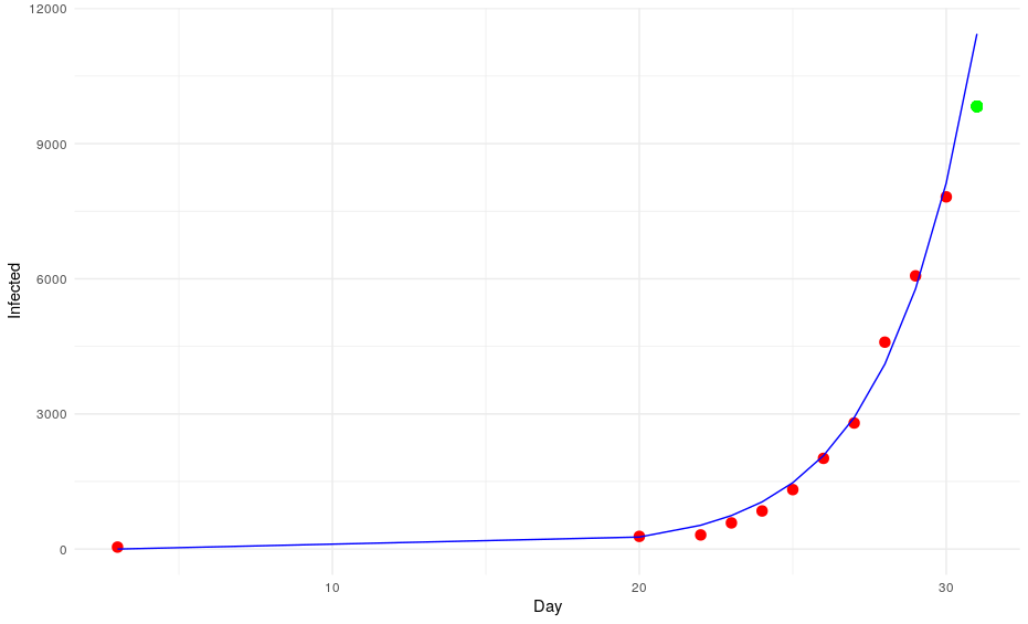
Okay, we have missed that one. Let’s put that number into the equation to try to predict the number of cases on day 32. The model says: 13996. However, the WHO says that there are 11953 infections (the blue point of the graph).

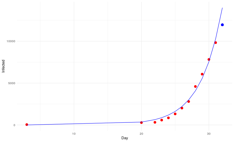
Again it seems that our model is overestimating the number of cases and although we are still in the uncertainty range (the standard error for a is almost half of its value: a = 0.72012; standard error of a = 0.33024), it is very likely that our exponential model will deviate more and more from the observations. In this case, I feel very relieved creating an inaccurate model, basically because the model predicts that by the end of April the entire human population would be infected.

The main reason for this simple model to fail is just that it does not take into account most of the factors that have an impact on the progression of the disease. It can’t predict how the disease would expand outside China, how it would progress in case of massive vaccinations, it doesn’t account for other human interventions such as quarantines, lockdowns or prevention measures, it doesn’t even take into account the number of deaths, natural or acquired immunity, etc…

Numerical simulations vs functions

So far we have created the most basic model, a model that takes into account just one parameter (time); however, as I have just mentioned, modeling infections requires introducing a lot of parameters into the equations; unfortunately, creating such multivariate functions can be so complex that in most of the cases it is not even possible from a practical point of view.

On the contrary, numerical simulations are simple but extremely powerful. We can add new constraints, parameters or elements with a couple of lines of code and they are so powerful that we could even simulate how a virus spreads to a new country based on the traveling rates or what would happen if a vaccine is found and we start vaccinating the population at a certain rate. As a counterpart, the simulations can be slow if we add too many elements or when simulating big populations.

Let’s see how we can create this type of simulations in R.

The first thing that we need to do is to create a vector to represent the population that we want to model:

#Parameters
Total_pop<-10000
df<-rep(1, Total_pop)

The elements of the vector represent the members of the population and the values the status of the subjects. In our case we assign 1 to non-infected but susceptible members, 0 to dead subjects, 2 to immune members and values > =3 represent infected members. As you can imagine you can expand this as much as you want just by adding new rules that you can check during the progression of the disease.

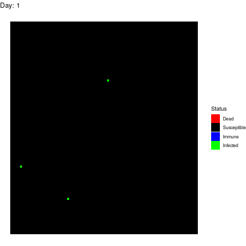
Now that we have our population, we can infect the patient-zero.

patient_zero<-sample(which(df==1),1)
df[patient_zero]<-3

So we can start tracking the progression of the disease with a for loop. In this case, I defined each iteration as a single day but you can change that to study quicker or slower processes.

for(i in 1:time){
  df[df>=3]<-df[df>=3]+1  

As you can see, the first thing that we do during each iteration (day) is to change the status of the infected by adding 1 to them, by doing this we can track differences in the patients during the progression of the disease (e.g. immunity, probability of recover/dead, infectivity, etc). Next, we find out how many people get infected each day. We compute that using two factors: the number of people in contact with each other and the probability of getting infected if you are contacted by an infected one.

for (k in 1:length(which(df>=3))) {
    round_contacts<-sample(which(df!=0),contact_rate)
    new_infected<-vector()
    for (l in 1:length(round_contacts)) {
      if(runif(1, min = 0, max = 1)<=Infection_rate & df[round_contacts[l]]==1) new_infected<-c(new_infected,round_contacts[l] )
      
    }
    new_infected<-length(new_infected)
    if(new_infected>0){
      
      if(length(which(df==1))<new_infected){
        new_infected<-length(which(df==1))
      }
    
    new_infected<-sample(which(df==1),new_infected)
    df[new_infected]<-3}
  }

The advantage of using these parameters is that it is possible to account for quarantines or more sparse areas/countries at the same time that we study the ability of the virus to propagate. In multivariate functions those parameters are combined into the famous R0 factor; however, as you can see we don’t need it here.

Next, we compute the number of deceased:

  #Deads
  infected<-which(df>=3)
  for (j in 1:length(infected)) {
    if(runif(1, min=0, max = 1)< ((1-Survival_rate)/silent_infection)) df[infected[j]]<-0
  }  

Then, we assume that patients get cured after surviving the virus for certain amount days and that from that day on, they become immune. In this particular model, these events happen in a deterministic way for simplicity reasons, but they can be computed as probabilities like the rest of factors (e.g. deads, infections, contacts).

if(length(which(df>=3+silent_infection))>0) df[which(df>=3+silent_infection)]<-2

Finally, we save the status of the population for each day as a row in a large matrix (progression[i,]<-df), so we can explore it when the simulation finishes.

And that’s it!! We are done!!

We can make this process much more complex by adding more constraints or more vectors to represent for instance other countries/cities with other densities/immune people but the core of the simulation is done. We only need to start playing around and plotting the results.

Simulations and inferences

The first thing that we need to do is to set the parameters that define the 2019-nCoV infection: We will simulate the infection for 100 days. The infection rate will be 1%, that means that 1% of the people that have suitable contacts with an infected people get the disease. In my opinion, this number is a good approximation considering an airborne transmission. Coronaviruses are heavy viruses when compared with other airborne viruses, the virus dies just after 2 hours outside the body and it only infects people through the nose, mouth or eyes. So it is not that likely that you are going to be infected from someone else easily. Next, we define the survival rate which so far seems to be around 97.7%. Then, we define the number of people that might have suitable contacts with an infected patient every day and 40 sounds like a reasonable number (You definitely cross by with 40 persons every day that might infect you: public transportation, workplace, elevators, family, etc…). Finally, it has been described that the patients can hold the virus for around 9 days without showing any symptoms. When we put all those parameters into the model we have that the R0 for our approximations (R0=3.6) is similar to the one described(2<R0<4).

All those parameters are defined here:

#Parameters
time<-100
Infection_rate<-0.01
Survival_rate<-0.9777
contact_rate<-40
silent_infection<-9

Now we run the simulation and prepare the data to be plotted:

df.plot<-expand.grid(c(1:100),c(1:100))
colnames(df.plot)<-c("X","Y")
df.plot$Time<-1
df.plot$Data<-progression[1,]

  for (i in 1:nrow(progression)) {
  dummy<-df.plot
  dummy$Time<-i
  dummy$Data<-progression[i,]
  if(!exists("to.plot")){
    to.plot<-dummy
  }else{
    to.plot<-rbind(to.plot,dummy)
  }
  }
  
  
to.plot$Data[to.plot$Data>=3]<-3

Scenario 1: No human intervention

Under this scenario, the virus propagates and the health authorities don’t do anything to stop it.

The virus spreads unstoppable and in the end, almost the entire population gets infected (and immune afterwards). This is obviously the worst-case scenario in terms of deads.

Scenario 2: Human efforts to contain the virus

Under this scenario, the healthcare authorities try to stop the infection by isolating the patients, by canceling classes in schools and universities and by locking down cities. These efforts reduce the number of suitable contacts from 40 to 10 (if you don’t go to class or you use a mask you are reducing the number of suitable contacts). The measurements start after 15 days from the first infection. We simulate this by adding this line to the loop:

  if(i>15) contact_rate<-10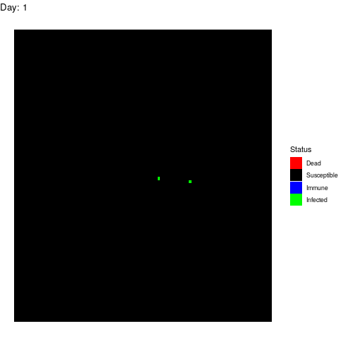

The virus propagates faster at the beggining but the efforts work and the the population gets immune while the infection rate decreases leading to an erradication of the virus.

Scenario 3. Vaccination of the population

Under this scenario, healthcare authorities develop a vaccine and start vaccinating the population at a rate of 200 persons per day.

In this very unlikely scenario (no matter what Hollywood says. It is impossible to develop and test a vaccine in 15 days), the virus expands quickly and some point it competes with the healthcare authorities, but since the number of infected patients is already very high, the immune individuals don’t outcompete the virus on the long term.

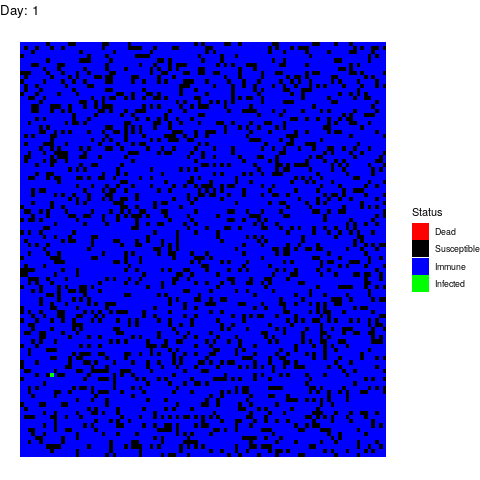
Bonus Scenario 4. Prior vaccination

I want to dedicate this scenario to the anti-vaccine movement: Let’s say that in a few years a vaccine is found and that certain government decides to vaccinate the population. However the vaccine is only able to prevent the disease in 90% of the patients by the time the virus strikes back:

As you can see, vaccines are effective not only avoiding the vaccinated people to get infected but also by isolating the susceptible population so the virus gets eradicated quickly.

Now, let’s imagine that 30% of the population refuses to get the vaccine afraid of turning autistic. In total, 40% of the population is sensitive.

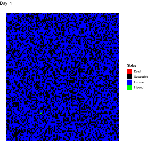
Luckily for the normal people, the virus doesn’t propagate too much but it is a pity that we haven’t found vaccines against stupidity yet because people die because of them.

The problem with this anti-vaccine movement is that the people that don’t get vaccinated compromise not only their security but the security of the people who took the vaccine but for whatever reason didn’t gain immunity.
This is the reason why vaccines should be mandatory for the population or at least mandatory to have any right to interact with other people: if you are not vaccinated you shouldn’t get a job, a ticket to use public transportations, tickets for concerts, etc…

Your rights (to not take a vaccine) end where mine (to be healthy) begin.

Conclusions

After all these simulations it seems that we might be facing scenario 2 in this particular case. So unless the virus mutates it will be eradicated in few months. Of course, these simulations are very very basic and there are a lot of elements that are not taken into account. Things like possible reservoirs (pangolins?), additional mutations, national borders, etc… are very relevant to simulate situations like this one. Additionally, we should establish all parameters as probability functions instead of deterministic ones.

With all those things clarified, I still think that this is a very powerful tool that can be used to explore different scenarios and to plan and evaluate different actions to stop the contagion.

Links of interest

WHO
CDC
nCoV19 LIVE
Source Code